b9cc3e3597f5fd9cc7861d3378ec7679.ppt
- Количество слайдов: 39
Risk Analysis November 3, 2008
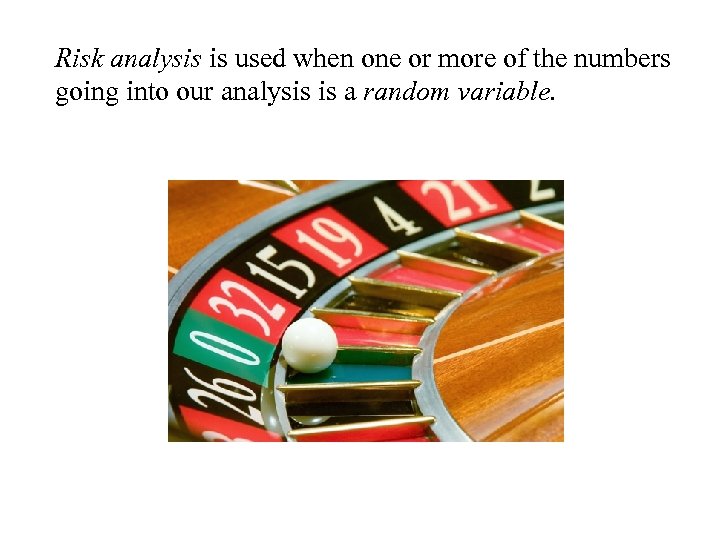
Risk analysis is used when one or more of the numbers going into our analysis is a random variable.
Random variables can be discrete – e. g. , the integer that comes up on a roulette wheel – or continuous, e. g. , the length of time we have to wait until our company starts showing a profit. Conventionally, we use a capital letter, such as `X’, to denote the variable, and a lower-case letter, such as `x 1’, to denote a particular value of that variable. So if X is the number that’s going to come up on the next spin of the wheel, x 1 = 1 is a possible value of X.
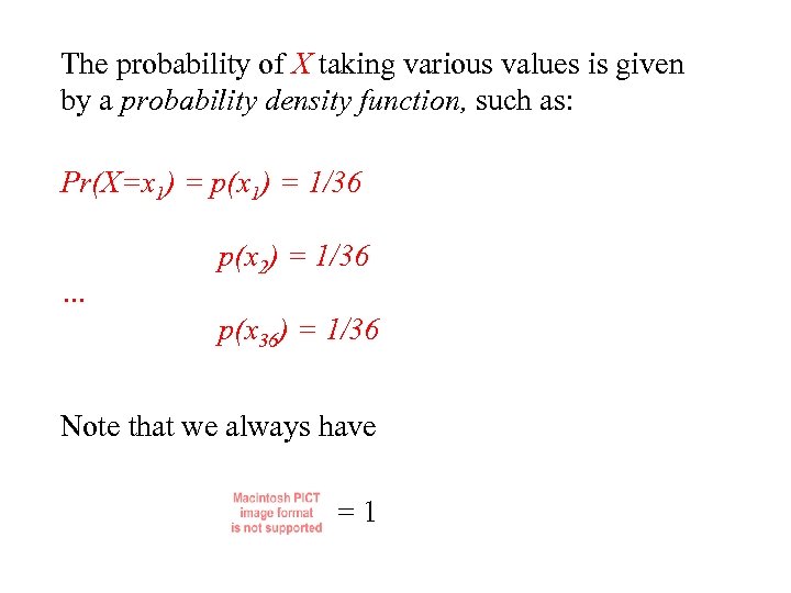
The probability of X taking various values is given by a probability density function, such as: Pr(X=x 1) = p(x 1) = 1/36 … p(x 2) = 1/36 p(x 36) = 1/36 Note that we always have =1
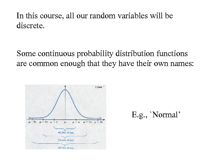
In this course, all our random variables will be discrete. Some continuous probability distribution functions are common enough that they have their own names: E. g. , `Normal’
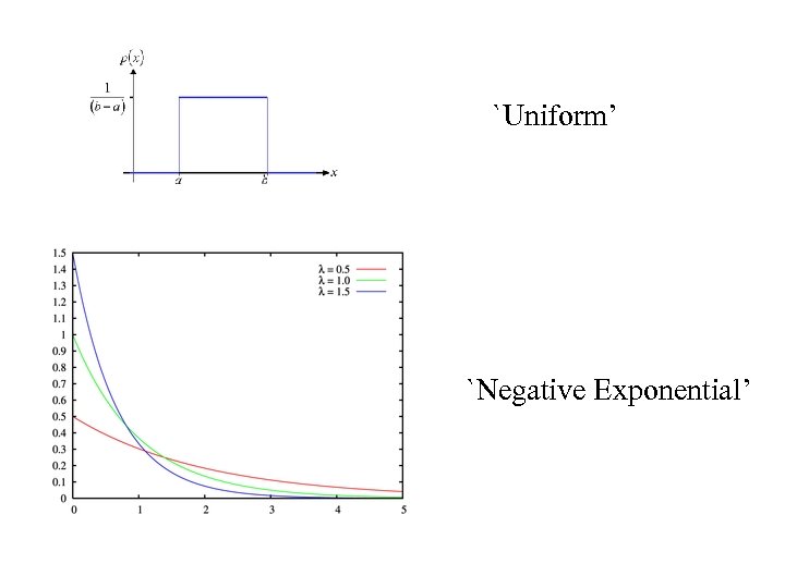
`Uniform’ `Negative Exponential’
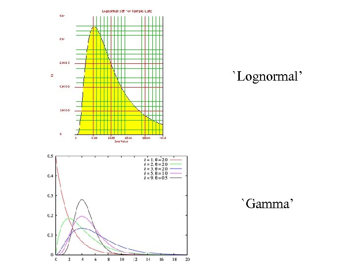
`Lognormal’ `Gamma’
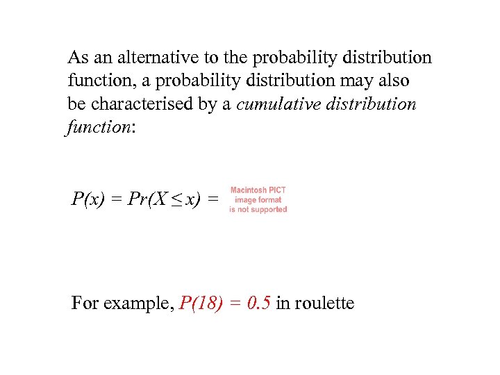
As an alternative to the probability distribution function, a probability distribution may also be characterised by a cumulative distribution function: P(x) = Pr(X ≤ x) = For example, P(18) = 0. 5 in roulette
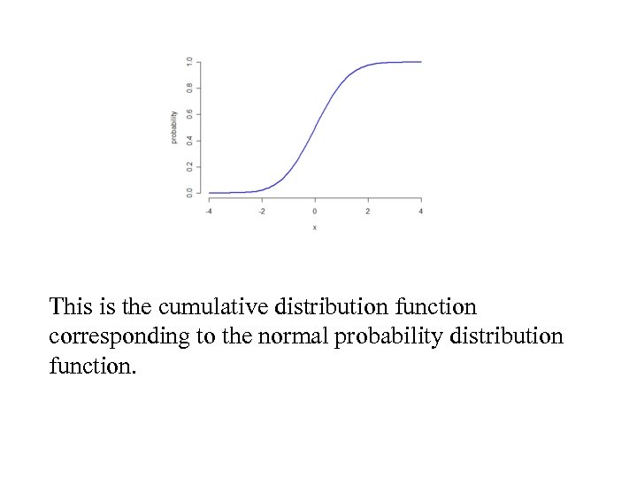
This is the cumulative distribution function corresponding to the normal probability distribution function.
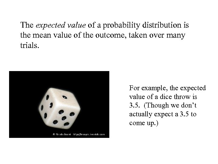
The expected value of a probability distribution is the mean value of the outcome, taken over many trials. For example, the expected value of a dice throw is 3. 5. (Though we don’t actually expect a 3. 5 to come up. )
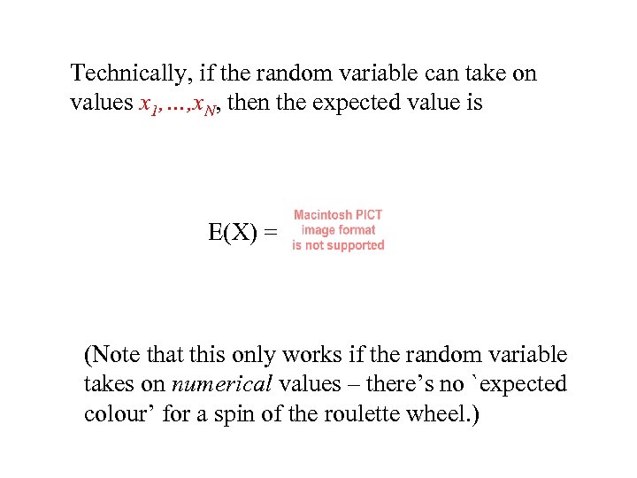
Technically, if the random variable can take on values x 1, …, x. N, then the expected value is E(X) = (Note that this only works if the random variable takes on numerical values – there’s no `expected colour’ for a spin of the roulette wheel. )
Simple example: We are doing research into a new product. There is a 50% chance the research will succeed by the end of next year, increasing profits by $100, 000, but if it fails, it will generate no income. How much is it worth spending on the research?
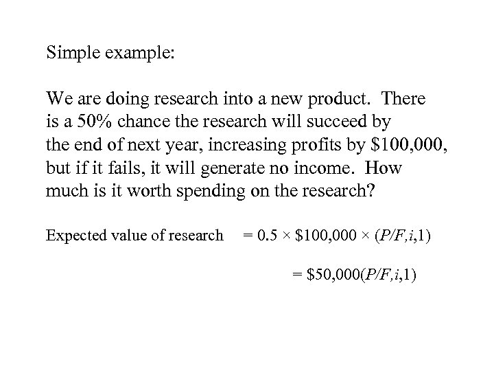
Simple example: We are doing research into a new product. There is a 50% chance the research will succeed by the end of next year, increasing profits by $100, 000, but if it fails, it will generate no income. How much is it worth spending on the research? Expected value of research = 0. 5 × $100, 000 × (P/F, i, 1) = $50, 000(P/F, i, 1)
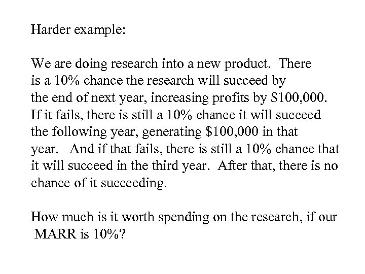
Harder example: We are doing research into a new product. There is a 10% chance the research will succeed by the end of next year, increasing profits by $100, 000. If it fails, there is still a 10% chance it will succeed the following year, generating $100, 000 in that year. And if that fails, there is still a 10% chance that it will succeed in the third year. After that, there is no chance of it succeeding. How much is it worth spending on the research, if our MARR is 10%?
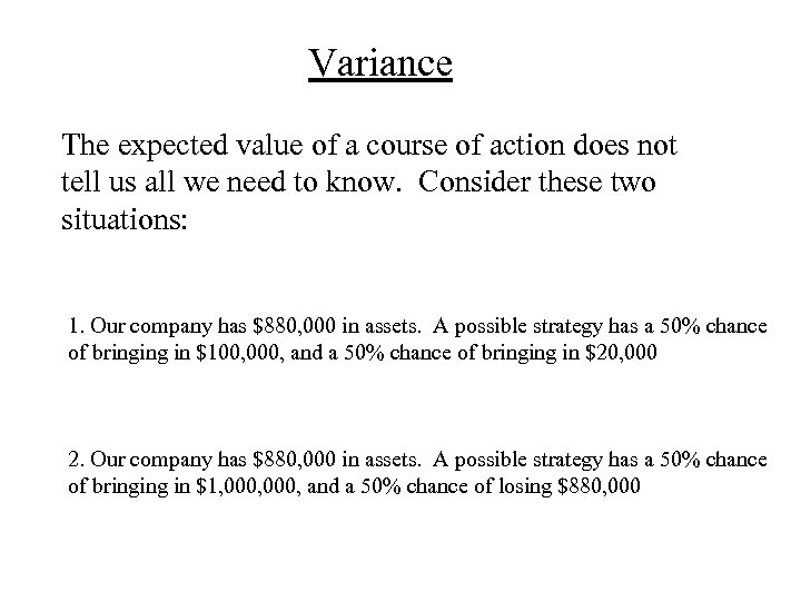
Variance The expected value of a course of action does not tell us all we need to know. Consider these two situations: 1. Our company has $880, 000 in assets. A possible strategy has a 50% chance of bringing in $100, 000, and a 50% chance of bringing in $20, 000 2. Our company has $880, 000 in assets. A possible strategy has a 50% chance of bringing in $1, 000, and a 50% chance of losing $880, 000
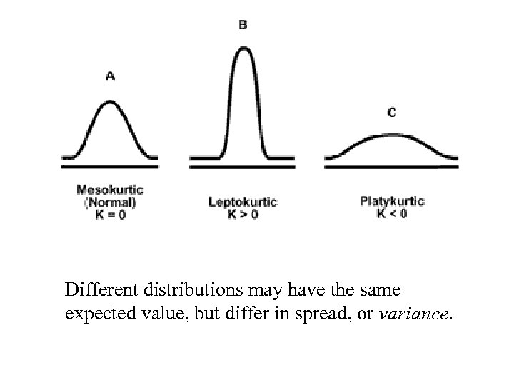
Different distributions may have the same expected value, but differ in spread, or variance.
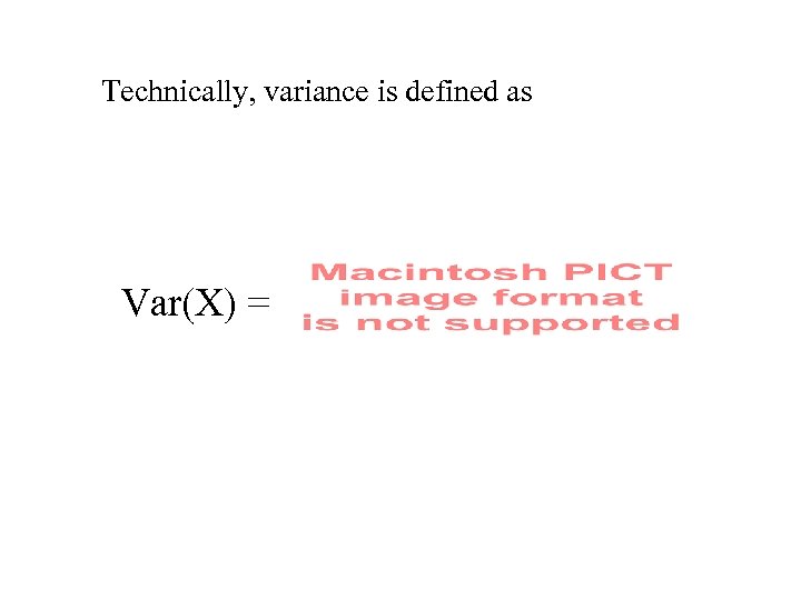
Technically, variance is defined as Var(X) =
In general, variance is bad. However, Las Vegas only exists because some people like high variance.
``Mean-Variance Dominance’’ Because most people prefer to reduce their variance, we say that one strategy is dominant over another if it has a higher mean and a lower variance. Alternatively, we say a strategy is efficient if no other strategy has both a higher mean and a lower variance.
What if we have more than one random variable in a problem? For example, we are planning a new product. Its manufacturing costs are expected to be $7, 000, plus or minus $1, 000. Its sales price will be $10, 000, and we are expecting to sell at least 40; there is a 50% chance we will sell at least 50, and a 10% chance we will sell more than 60. What are our expected profits?
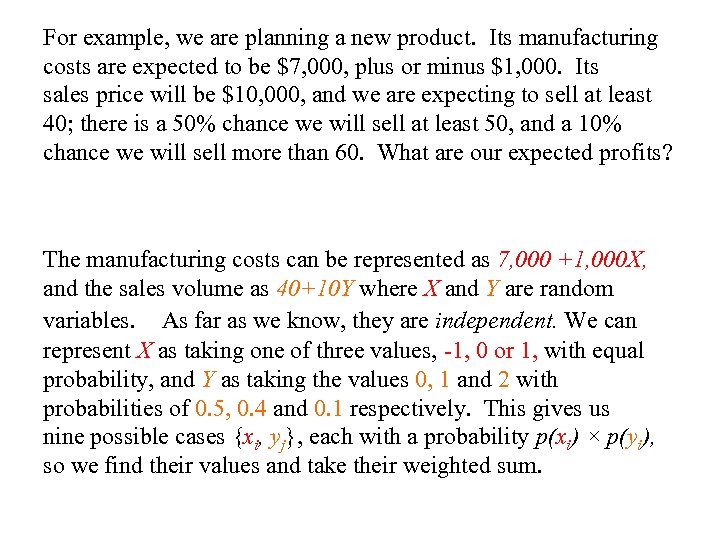
For example, we are planning a new product. Its manufacturing costs are expected to be $7, 000, plus or minus $1, 000. Its sales price will be $10, 000, and we are expecting to sell at least 40; there is a 50% chance we will sell at least 50, and a 10% chance we will sell more than 60. What are our expected profits? The manufacturing costs can be represented as 7, 000 +1, 000 X, and the sales volume as 40+10 Y where X and Y are random variables. As far as we know, they are independent. We can represent X as taking one of three values, -1, 0 or 1, with equal probability, and Y as taking the values 0, 1 and 2 with probabilities of 0. 5, 0. 4 and 0. 1 respectively. This gives us nine possible cases {xi, yj}, each with a probability p(xi) × p(yi), so we find their values and take their weighted sum.
More commonly, the unknowns in our calculation will be interdependent, not independent. To keep track of these, we need a decision tree.
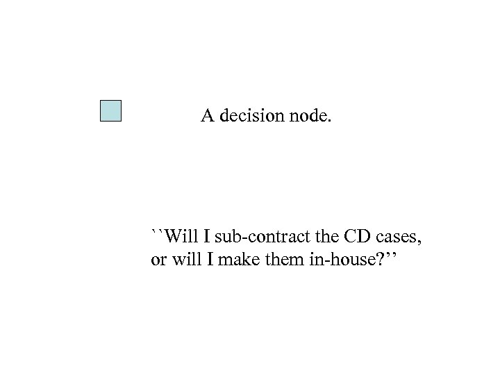
A decision node. ``Will I sub-contract the CD cases, or will I make them in-house? ’’
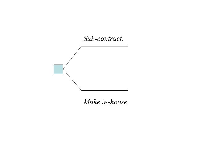
Sub-contract. Make in-house.
A chance node. ``If I produce the CD cases in –house, there’s a 50% chance I’ll run short of money. Then I’d have to borrow more, which would push my MARR from 10% to 12%. ’’
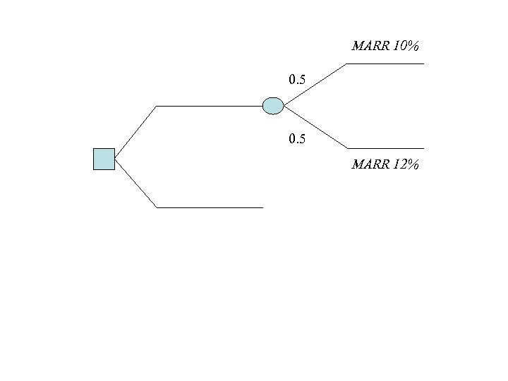
MARR 10% 0. 5 MARR 12%
A chance node. ``On the other hand, if I outsource there’s a 10% chance the subcontractor will be late, which will cost me $10, 000. ’’
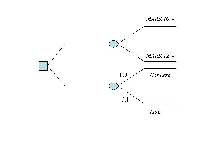
MARR 10% MARR 12% 0. 9 Not Late 0. 1 Late
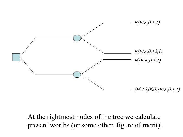
F(P/F, 0. 1, 1) F(P/F, 0. 12, 1) F/(P/F, 0. 1, 1) (F/-10, 000)(P/F, 0. 1, 1) At the rightmost nodes of the tree we calculate present worths (or some other figure of merit).
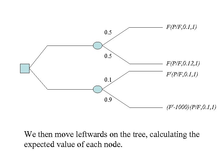
0. 5 F(P/F, 0. 1, 1) 0. 5 F(P/F, 0. 12, 1) 0. 1 F/(P/F, 0. 1, 1) 0. 9 (F/-1000)(P/F, 0. 1, 1) We then move leftwards on the tree, calculating the expected value of each node.
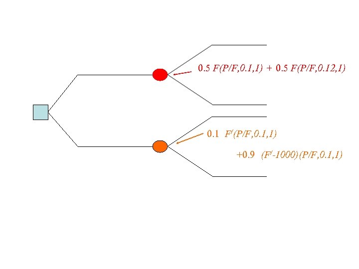
0. 5 F(P/F, 0. 1, 1) + 0. 5 F(P/F, 0. 12, 1) 0. 1 F/(P/F, 0. 1, 1) +0. 9 (F/-1000)(P/F, 0. 1, 1)
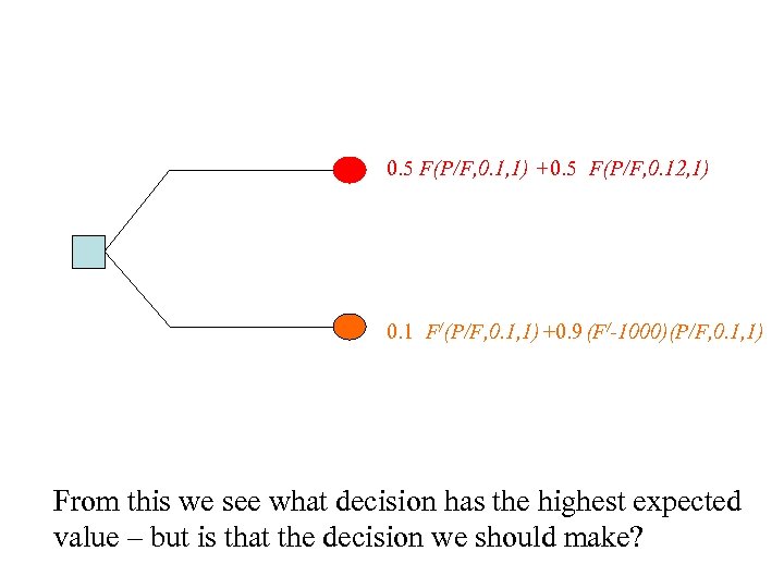
0. 5 F(P/F, 0. 1, 1) + 0. 5 F(P/F, 0. 12, 1) 0. 1 F/(P/F, 0. 1, 1) +0. 9 (F/-1000)(P/F, 0. 1, 1) From this we see what decision has the highest expected value – but is that the decision we should make?
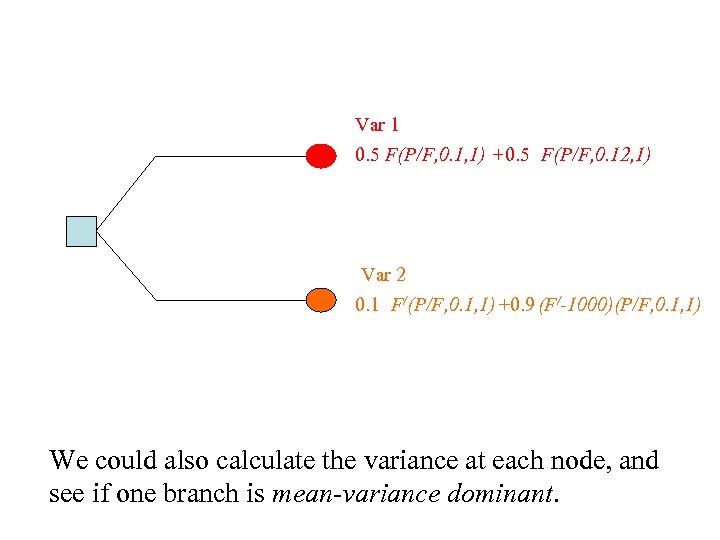
Var 1 0. 5 F(P/F, 0. 1, 1) + 0. 5 F(P/F, 0. 12, 1) Var 2 0. 1 F/(P/F, 0. 1, 1) +0. 9 (F/-1000)(P/F, 0. 1, 1) We could also calculate the variance at each node, and see if one branch is mean-variance dominant.
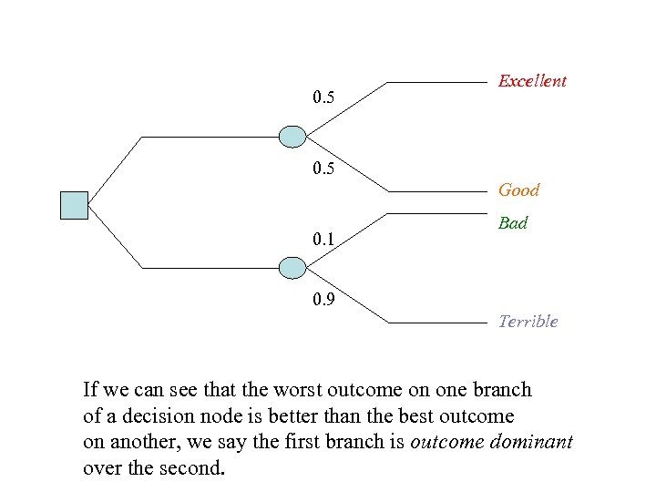
0. 5 Excellent 0. 5 Good 0. 1 Bad 0. 9 Terrible If we can see that the worst outcome on one branch of a decision node is better than the best outcome on another, we say the first branch is outcome dominant over the second.
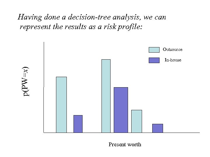
Having done a decision-tree analysis, we can represent the results as a risk profile: Outsource p(PW=x) In-house Present worth
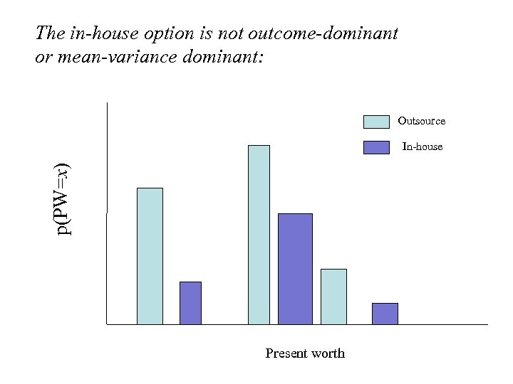
The in-house option is not outcome-dominant or mean-variance dominant: Outsource p(PW=x) In-house Present worth
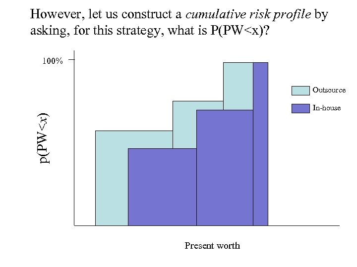
However, let us construct a cumulative risk profile by asking, for this strategy, what is P(PW<x)? 100% Outsource p(PW<x) In-house Present worth
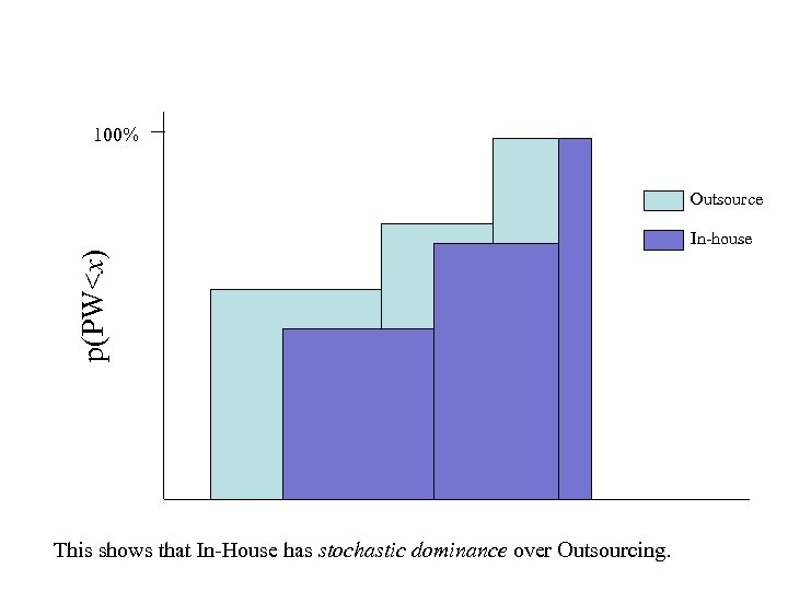
100% Outsource p(PW<x) In-house This shows that In-House has stochastic dominance over Outsourcing.
Example: we have a machine which may break down at any time over the next three years. We can replace it now, at a cost of $40, 000, or we can keep it in service till it breaks. That will cost us $10, 000 in lost production, and we will have to pay to have it replaced. Every year, there is a 30% chance that the cost of a replacement will go up by $5, 000, though we don’t expect there to be more than one such increase in the next three years. Our MARR is 20%.
b9cc3e3597f5fd9cc7861d3378ec7679.ppt