3190ea37b1f64c92229ca4077e7057e7.ppt
- Количество слайдов: 58


Review last lectures
 governor 1788 Picture shows an operation principle of the fly-ball (centrifugal) speed")
centrifugal (fly-ball) governor 1788 Picture shows an operation principle of the fly-ball (centrifugal) speed governor developed by James Watt.

simple feedback system heat transfer Qout desired temperature _ Qin thermostat switch air con + S room temperature office room
 system error or actuating signal input or reference summing junction or comparator")
closed-loop (feedback) system error or actuating signal input or reference summing junction or comparator input filter (transducer) + _ S controller disturbance plant control signal actuator process sensor or output transducer sensor noise output or controlled variable

closed-loop system advantages n n high accuracy not sensitive on disturbance controllable transient response controllable steady state error disadvantages n n n more complex more expensive possibility of instability recalibration needed need for output measurement
 disturbance plant controller control signal actuator")
open-loop system input or reference input filter (transducer) disturbance plant controller control signal actuator output or controlled variable process

open-loop system advantages n n n simple construction ease of maintenance less expensive no stability problem no need for output measurement disadvantages disturbances cause errors n changes in calibration cause errors n output may differ from what is desired n recalibration needed n

Example 1: Liquid Level System Goal: Design the input valve control to maintain a constant height regardless of the setting of the output valve (input flow) Input valve control float (resistance) (height) (output flow) (volume) Output valve

Example 2: Admission Control Users Goal: Design the controller to maintain a constant queue length regardless of the workload RPCs Reference value Administrator Controller Tuning control Sensor Server Queue Length Server Log

Why Control Theory n Systematic approach to analysis and design • • n Transient response Consider sampling times, control frequency Taxonomy of basic controls Select controller based on desired characteristics Predict system response to some input • Speed of response (e. g. , adjust to workload changes) • Oscillations (variability) n Approaches to assessing stability and limit cycles

Controller Design Methodology Start System Modeling Controller Design Block diagram construction Controller Evaluation Transfer function formulation and validation Objective achieved ? N Model Ok? Y N Y Stop

Control System Goals n Regulation • thermostat, target service levels n Tracking • robot movement, adjust TCP window to network bandwidth n Optimization • best mix of chemicals, minimize response times

Approaches to System Modelling n First Principles • Based on known laws n Physics, Queuing theory • Difficult to do for complex systems n Experimental (System ID) • Statistical/data-driven models • Requires data • Is there a good “training set”?
 is defined")
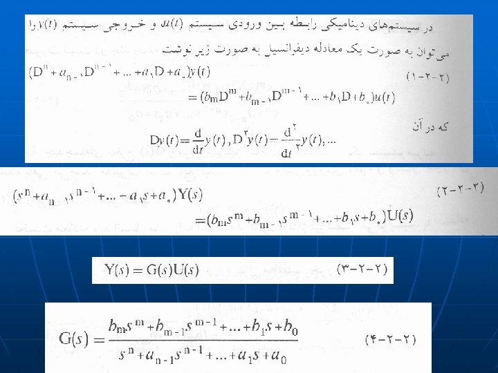
Laplace transforms n n n The Laplace transform of a signal f(t) is defined as The Laplace transform is an integral transform that changes a function of t to a function of a complex variable s = s + jw The inverse Laplace transform changes the function of s back to a function of t
 Unit impulse d (t ) Unit")
Laplace transforms of basic functions f (t ) Unit impulse d (t ) Unit step u (t ) Exponential e−at Sine wave sin(t) Cosine wave cos(t) Polynomial tn e−at x(t) Note: f(t) = 0, t < 0 F (s )
 Laplace transform: signal 1 t 0 w s")
Example f (t) Laplace transform: signal 1 t 0 w s

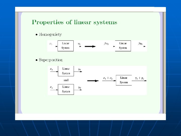
Properties of Laplace transforms n Linear operator: if and then for any two signals n f 1(t) and f 2(t) and any two constants a 1 and a 2 Time delay:

Properties of Laplace transforms cont. n Laplace transforms of derivatives: if then

Properties of Laplace transforms cont. n n Laplace transform of integrals: The Laplace transform changes differential equations in t into arithmetic equations in s

Laplace Transform Properties

Using Laplace transforms to solve ODEs n n 1. 2. 3. n The Laplace transform can be used to solve differential equations Method: Transform the differential equation into the ‘Laplace domain’ (equation in t → equation in s) Rearrange to get the solution Transform the solution back from the Laplace domain to the time domain (signal in s → signal in t) Usually the Laplace transform (step 1) and the inverse transform (step 3) are done using a Table of Laplace transforms

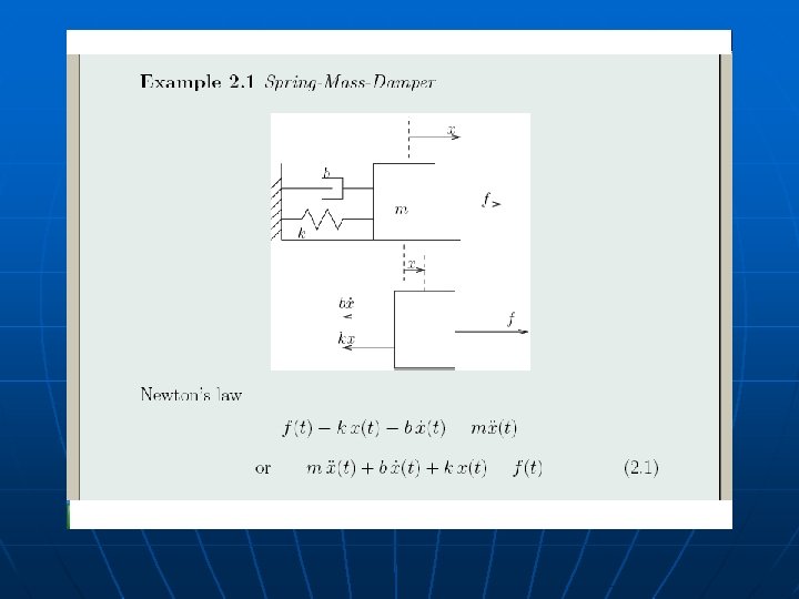
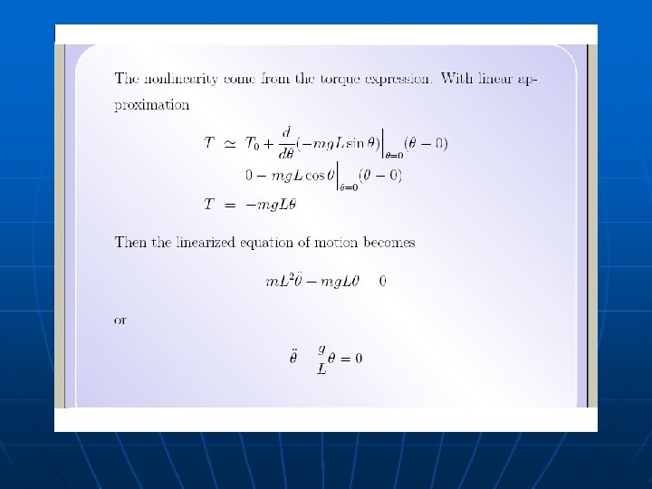
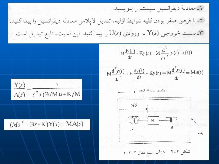
Example n Use Laplace transforms to find the unforced response of a spring-mass-damper with initial conditions x k m = 1 kg k = 2 N/m b = 3 Ns/m f m b x Equation of motion m Free body diagram f

Example – solution n n Take Laplace transform of both sides of equation of motion: Equation of motion in Laplace domain is

n Rearrange: External force n Initial conditions The system can be in motion if 1. An external force is applied 2. The initial conditions are not an equilibrium state (not zero) n Apply initial conditions:

n n n Partial fraction expansion: Use tables to find inverse Laplace transform System response (in time domain) is x(t) x 0 0 t

Partial fraction expansion n n A partial fraction expansion can be used to find the inverse transform of This can be expanded as Note that So

Example - Partial fraction expansion n Find the partial fraction expansion of n This can be expanded as n So

Other examples 1. 2. 3.
 • Value")
Insights from Laplace Transforms n What the Laplace Transform says about f(t) • Value of f(0) n Initial value theorem • Does f(t) converge to a finite value? n Poles of F(s) • Does f(t) oscillate? n Poles of F(s) • Value of f(t) at steady state (if it converges) n Limiting value of F(s) as s ---> 0
 = Y(s) / X(s) n n n X(s)")
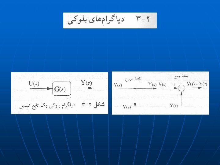
Transfer Function n Definition • H(s) = Y(s) / X(s) n n n X(s) H(s) Y(s) Relates the output of a linear system (or component) to its input Describes how a linear system responds to an impulse All linear operations allowed • Scaling, addition, multiplication

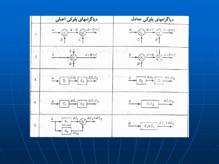
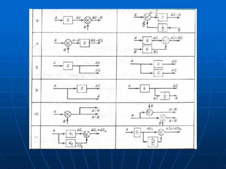
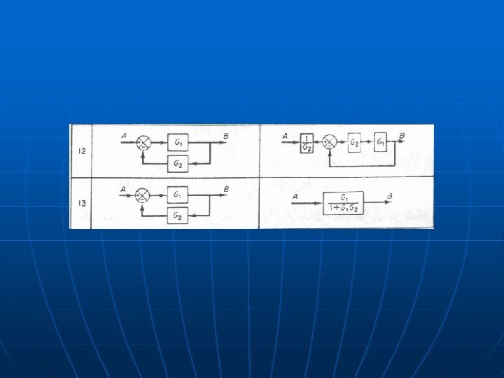
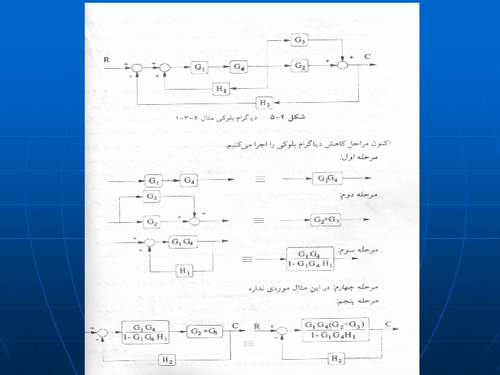
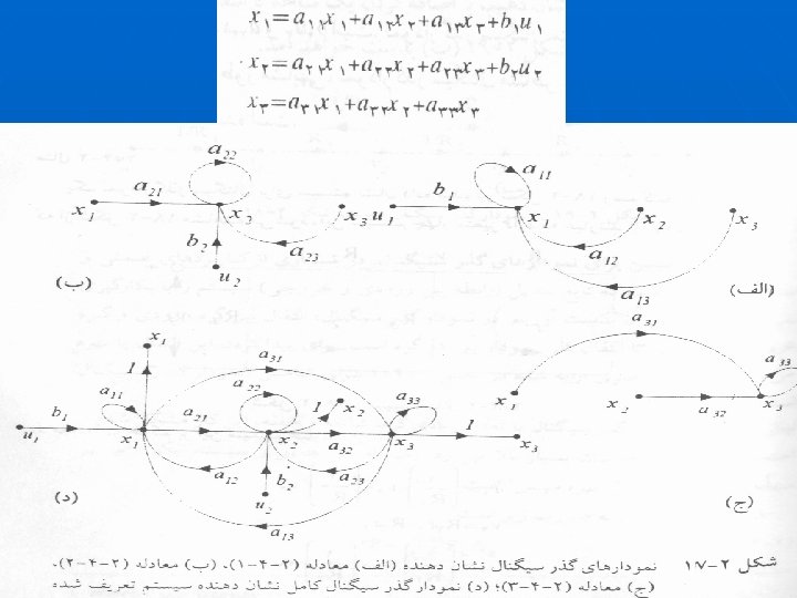
Block Diagrams n n n Pictorially expresses flows and relationships between elements in system Blocks may recursively be systems Rules • Cascaded (non-loading) elements: convolution • Summation and difference elements n Can simplify

Block Diagram of System Disturbance Reference Value + S Controller S – Transducer Plant

Combining Blocks Reference Value + S Combined Block – Transducer

Key Transfer Functions Reference S + Plant Controller – Transducer

Class Home page: http: //saba. kntu. ac. ir/eecd/People/aliyari/
3190ea37b1f64c92229ca4077e7057e7.ppt