Review ESD 260 Fall 2003 1 Demand

Review ESD. 260 Fall 2003 1

Demand Forecasting 2

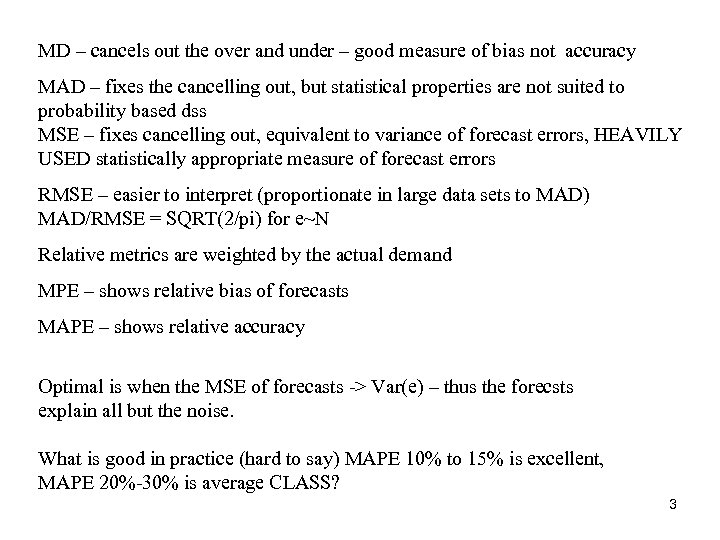MD – cancels out the over and under – good measure of bias not accuracy MAD – fixes the cancelling out, but statistical properties are not suited to probability based dss MSE – fixes cancelling out, equivalent to variance of forecast errors, HEAVILY USED statistically appropriate measure of forecast errors RMSE – easier to interpret (proportionate in large data sets to MAD) MAD/RMSE = SQRT(2/pi) for e~N Relative metrics are weighted by the actual demand MPE – shows relative bias of forecasts MAPE – shows relative accuracy Optimal is when the MSE of forecasts -> Var(e) – thus the forecsts explain all but the noise. What is good in practice (hard to say) MAPE 10% to 15% is excellent, MAPE 20%-30% is average CLASS? 3

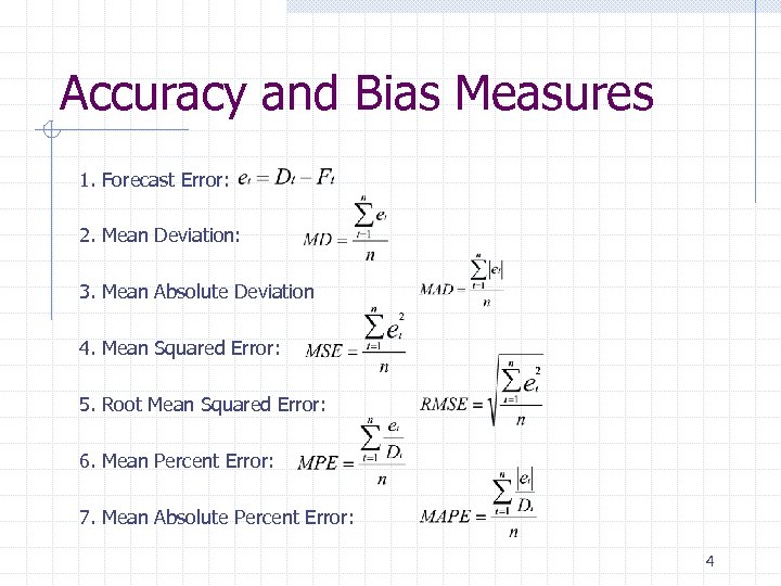Accuracy and Bias Measures 1. Forecast Error: 2. Mean Deviation: 3. Mean Absolute Deviation 4. Mean Squared Error: 5. Root Mean Squared Error: 6. Mean Percent Error: 7. Mean Absolute Percent Error: 4

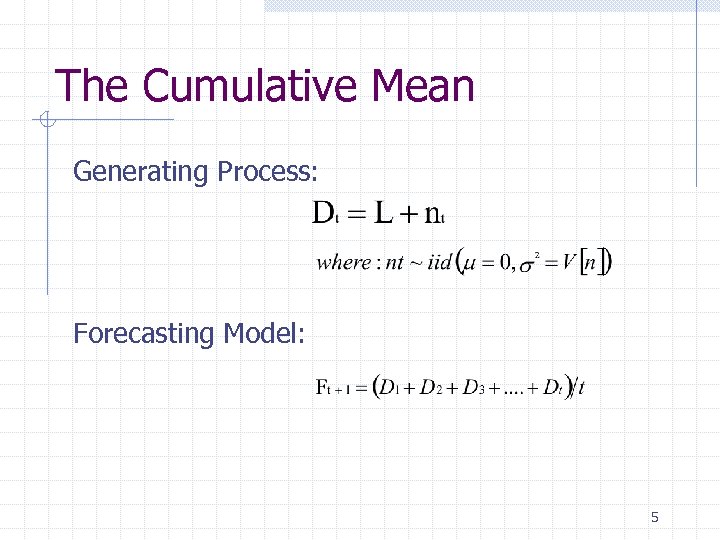The Cumulative Mean Generating Process: Forecasting Model: 5

Stationary model – mean does not change – pattern is a constant Not used in practice – is anything constant? Thought though is to use as large a sample si. De as possible to 6

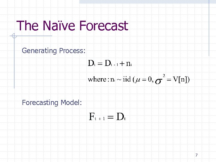The Naïve Forecast Generating Process: Forecasting Model: 7

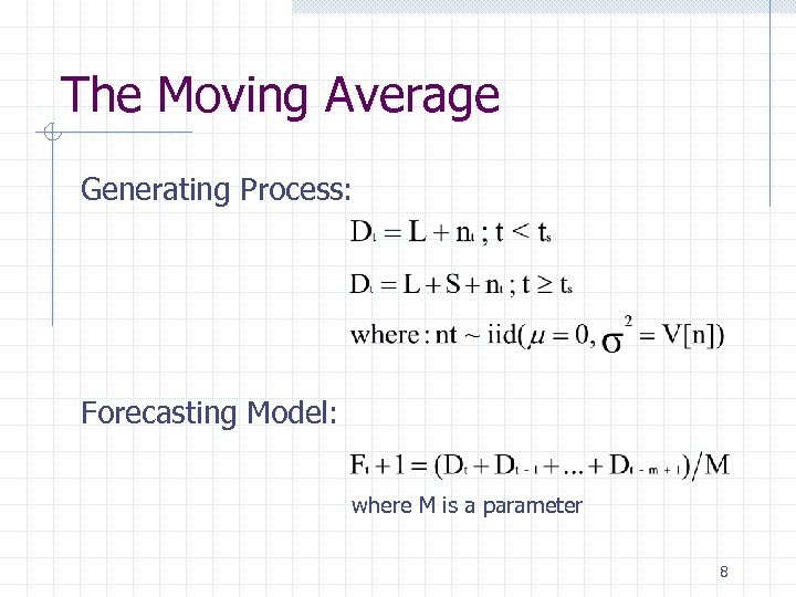The Moving Average Generating Process: Forecasting Model: where M is a parameter 8

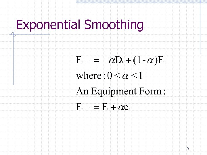Exponential Smoothing 9

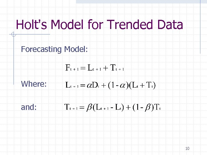Holt's Model for Trended Data Forecasting Model: Where: and: 10

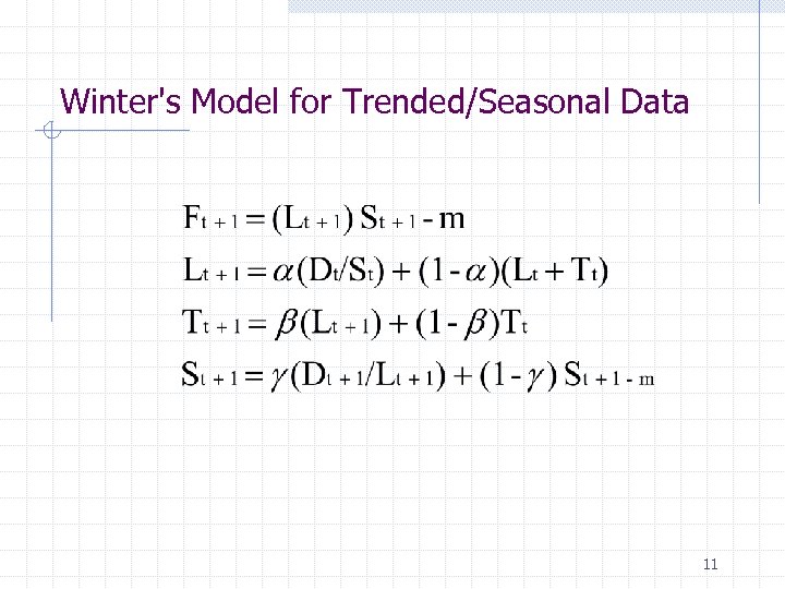Winter's Model for Trended/Seasonal Data 11

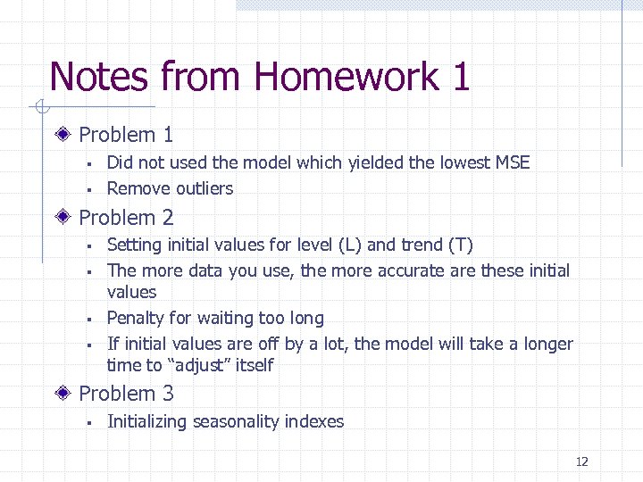Notes from Homework 1 Problem 1 § § Did not used the model which yielded the lowest MSE Remove outliers Problem 2 § § Setting initial values for level (L) and trend (T) The more data you use, the more accurate are these initial values Penalty for waiting too long If initial values are off by a lot, the model will take a longer time to “adjust” itself Problem 3 § Initializing seasonality indexes 12

Inventory Management 13

Bottomline Inventory is not bad. Inventory is good. Inventory is an important tool which, when correctly used, can reduce total cost and improve the level of service performance in a logistics system. 14

Fundamental Purpose of Inventory To Reduce Total System Cost § To buffer uncertainties in: - supply, - demand, and/or - transportation the firm carries safety stocks. § To capture scale economies in: - purchasing, - production, and/or - Transportation the firm carries cycle stocks. 15

Dimensions of Inventory Modeling Demand § § § Constant vs Variable Known vs Random Continuous vs Discrete Lead time § § Instantaneous Constant or Variable (deterministic/stochastic) Dependence of items § § § Independent Correlated Indentured Review Time § § Continuous Periodic Discounts § § None All Units or Incremental Excess Demand § § None All orders are backordered Lost orders Substitution Perishability § § None Uniform with time Planning Horizon § § § Single Period Finite Period Infinite 16

Lot sizing 17

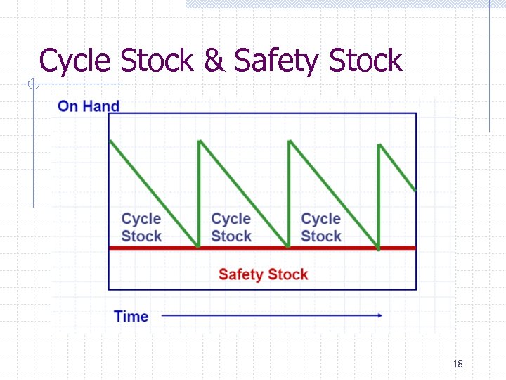Cycle Stock & Safety Stock 18

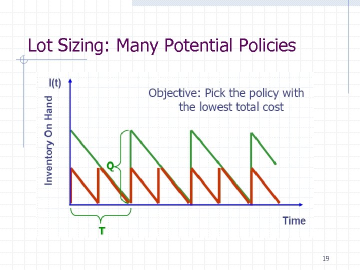Lot Sizing: Many Potential Policies 19

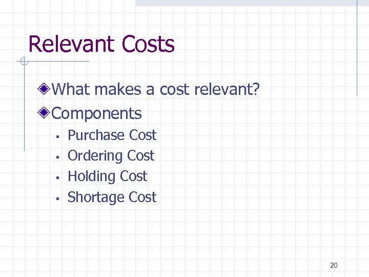Relevant Costs What makes a cost relevant? Components § § Purchase Cost Ordering Cost Holding Cost Shortage Cost 20

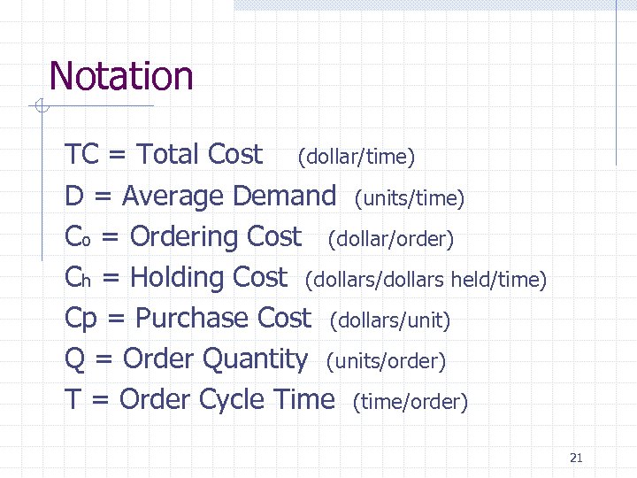Notation TC = Total Cost (dollar/time) D = Average Demand (units/time) Co = Ordering Cost (dollar/order) Ch = Holding Cost (dollars/dollars held/time) Cp = Purchase Cost (dollars/unit) Q = Order Quantity (units/order) T = Order Cycle Time (time/order) 21

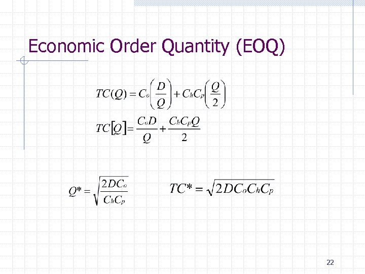Economic Order Quantity (EOQ) 22

From TC [Q] to Q* Take the derivate and set it to 0 23

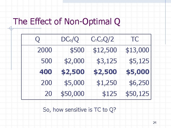The Effect of Non-Optimal Q Q DCo/Q Ch. Cp. Q/2 TC 2000 $500 $12, 500 $13, 000 500 $2, 000 $3, 125 $5, 125 400 $2, 500 $5, 000 200 $5, 000 $1, 250 $6, 250 20 $50, 000 $125 $50, 125 So, how sensitive is TC to Q? 24

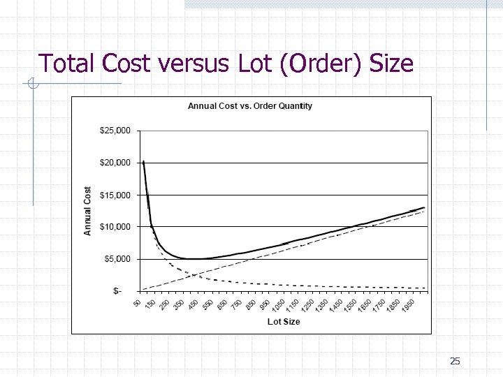Total Cost versus Lot (Order) Size 25

Minimum point is relatively flat : there is a range / small changes in parameters may change the optimal Q 26

Insights from EOQ There is a direct trade off between lot size and total inventory Total cost is relatively insensitive to changes § Very robust with respect to changes in: § Q – rounding of order quantities § D – errors in forecasting § Ch, Co, Cp– errors in cost parameters Thus, EOQ is widely used despite its highly restrictive assumptions 27

Introduce Discounts to Lot Sizing Types of discounts § § § All units discount Incremental discount One time only discount How will different discounting strategies impact your lot sizing decision? 28

All Units Discount Unit Price [Cpi] Price Break Quantity [PBQI] $50. 00 0 $45. 00 500 $40. 00 1000 29

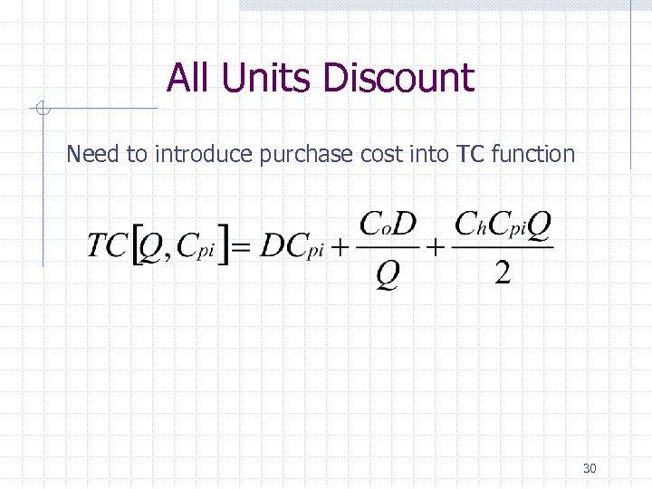All Units Discount Need to introduce purchase cost into TC function 30

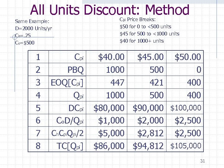All Units Discount: Method Cpi Price Breaks: $50 for 0 to <500 units $45 for 500 to <1000 units $40 for 1000+ units Same Example: D=2000 Units/yr Ch=. 25 Co=$500 1 2 3 4 5 6 7 8 Cpi PBQ EOQ[Cpi] Qpi DCpi Co. D/Qpi Ch. Cpi. Qpi/2 TC[Qpi] $40. 00 $45. 00 $50. 00 1000 500 0 447 421 400 1000 500 400 $80, 000 $90, 000 $100, 000 $1, 000 $2, 500 $5, 000 $2, 812 $2, 500 $86, 000 $94, 812 $105, 000 31

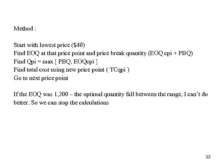Method : Start with lowest price ($40) Find EOQ at that price point and price break quantity (EOQ cpi + PBQ) Find Qpi = max [ PBQ, EOQcpi ] Find total cost using new price point ( TCqpi ) Go to next price point If the EOQ was 1, 200 – the optimal quantity fall between the range, I can’t do better. So we can stop the calculations 32

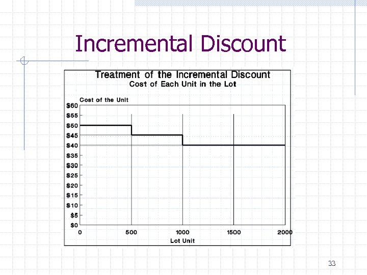Incremental Discount 33

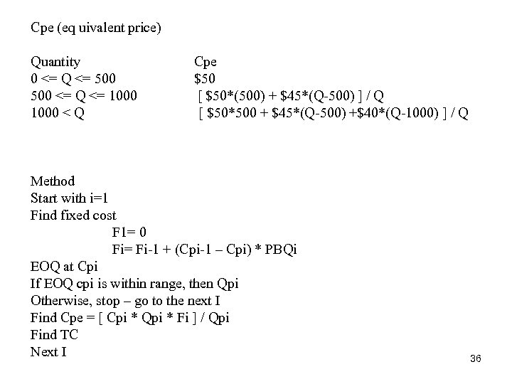
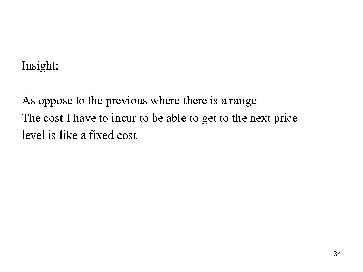Insight: As oppose to the previous where there is a range The cost I have to incur to be able to get to the next price level is like a fixed cost 34

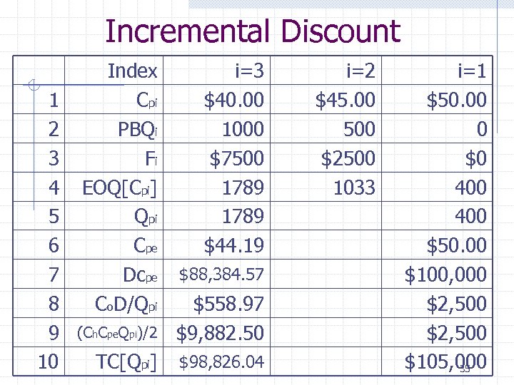Incremental Discount 1 2 3 4 5 6 7 8 9 10 Index Cpi PBQi Fi EOQ[Cpi] Qpi Cpe Dcpe Co. D/Qpi i=3 $40. 00 1000 $7500 1789 $44. 19 $88, 384. 57 (Ch. Cpe. Qpi)/2 $558. 97 $9, 882. 50 TC[Qpi] $98, 826. 04 i=2 $45. 00 500 $2500 1033 i=1 $50. 00 0 $0 400 $50. 00 $100, 000 $2, 500 $105, 000 35

Cpe (eq uivalent price) Quantity 0 <= Q <= 500 <= Q <= 1000 < Q Cpe $50 [ $50*(500) + $45*(Q-500) ] / Q [ $50*500 + $45*(Q-500) +$40*(Q-1000) ] / Q Method Start with i=1 Find fixed cost F 1= 0 Fi= Fi-1 + (Cpi-1 – Cpi) * PBQi EOQ at Cpi If EOQ cpi is within range, then Qpi Otherwise, stop – go to the next I Find Cpe = [ Cpi * Qpi * Fi ] / Qpi Find TC Next I 36

One Time Discount 37

Similar to a price increase where we order more right before the price increase 38

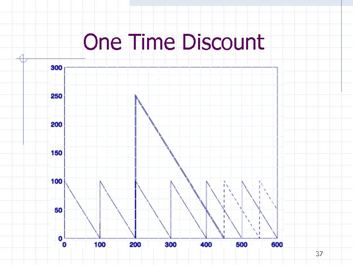
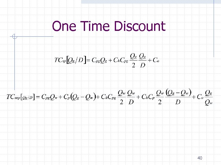
One Time Discount Let, § § § Cpg = One time deal purchase price ($/unit) Qg = One time special order quantity (units) TCsp=TC over time covered by special purchase ($) Then, 39

One Time Discount 40

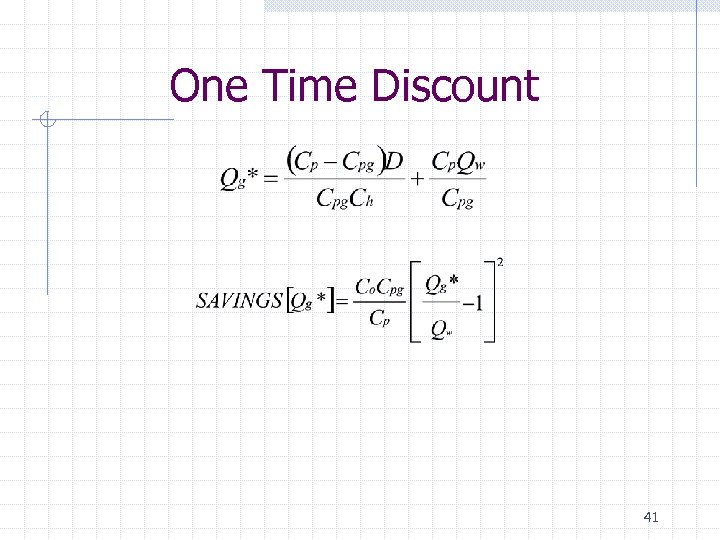One Time Discount 41

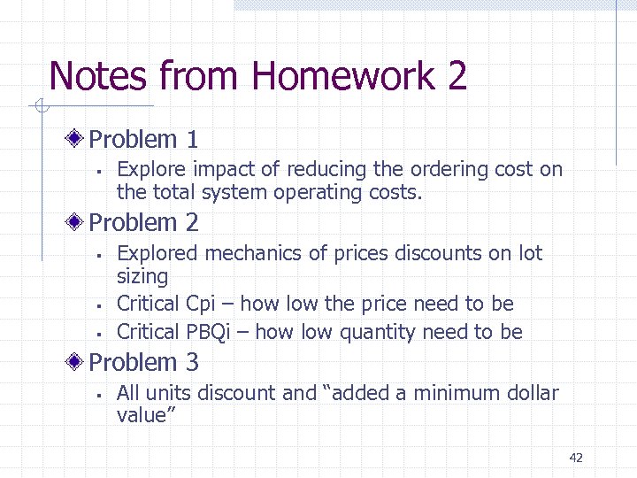Notes from Homework 2 Problem 1 § Explore impact of reducing the ordering cost on the total system operating costs. Problem 2 § § § Explored mechanics of prices discounts on lot sizing Critical Cpi – how low the price need to be Critical PBQi – how low quantity need to be Problem 3 § All units discount and “added a minimum dollar value” 42

Safety Stock 43

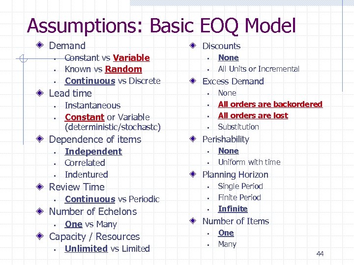Assumptions: Basic EOQ Model Demand § § § Constant vs Variable Known vs Random Continuous vs Discrete Lead time § § Instantaneous Constant or Variable (deterministic/stochastc) Dependence of items § § § Independent Correlated Indentured Review Time § Continuous vs Periodic Number of Echelons § One vs Many Capacity / Resources § Unlimited vs Limited Discounts § § None All Units or Incremental Excess Demand § § None All orders are backordered All orders are lost Substitution Perishability § § None Uniform with time Planning Horizon § § § Single Period Finite Period Infinite Number of Items § § One Many 44

Fundamental Purpose of Inventory Firm carries safety stock to buffer uncertainties in: - supply, - demand, and/or - transportation 45

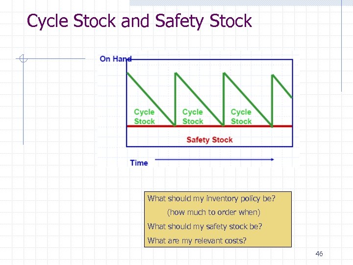Cycle Stock and Safety Stock What should my inventory policy be? (how much to order when) What should my safety stock be? What are my relevant costs? 46

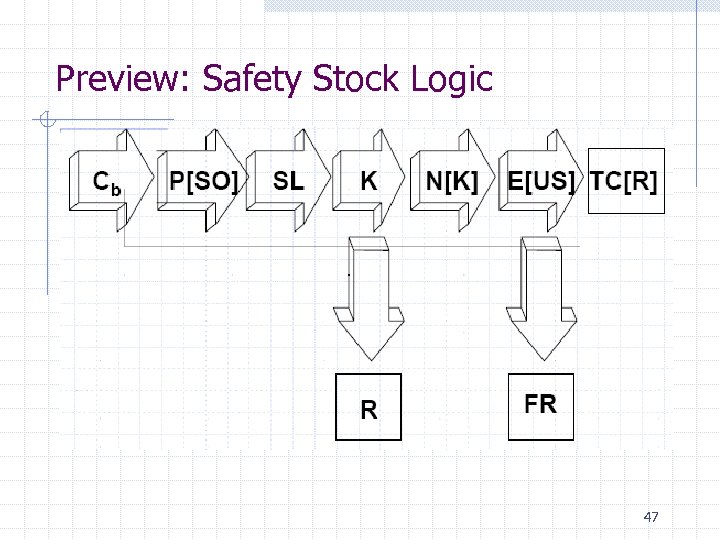Preview: Safety Stock Logic 47

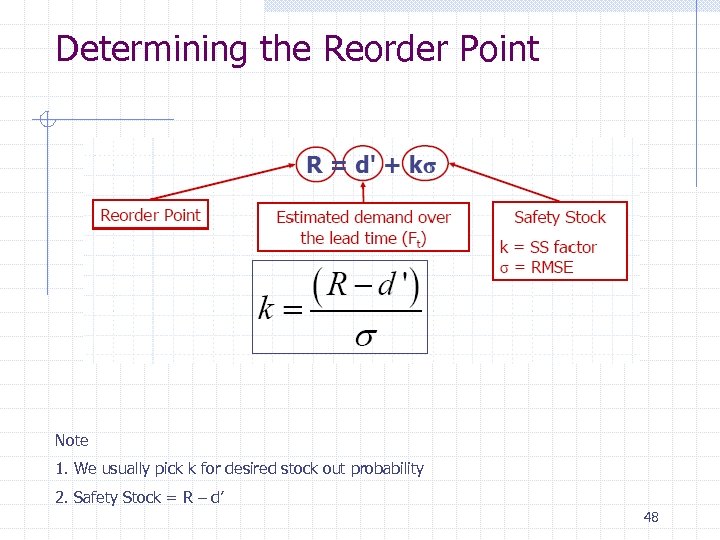Determining the Reorder Point Note 1. We usually pick k for desired stock out probability 2. Safety Stock = R – d’ 48

Define Some Terms Safety Stock Factor (k) Amount of inventory required in terms of standard deviations worth of forecast error Stockout Probability = P[d > R] The probability of running out of inventory during lead time Service Level = P[d ≤ R] = 1 -P[SO] The probability of NOT running out of inventory during lead time 49

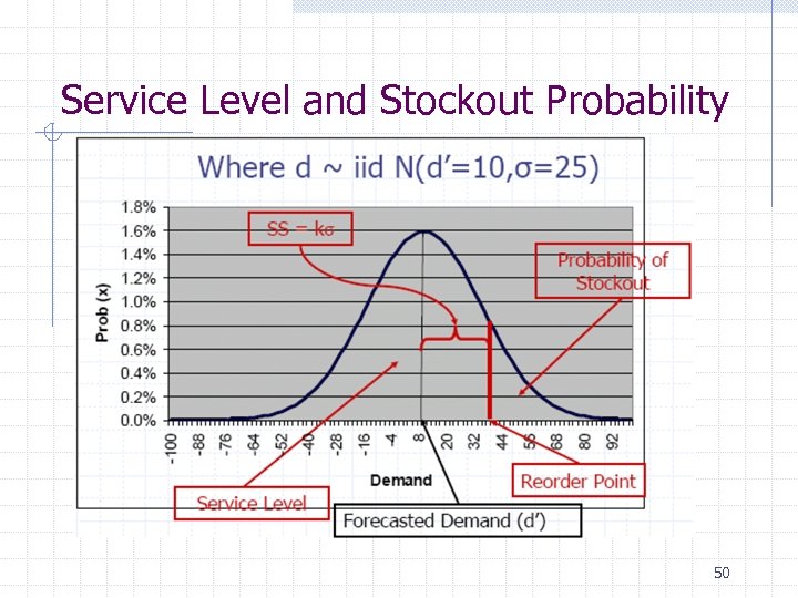Service Level and Stockout Probability 50

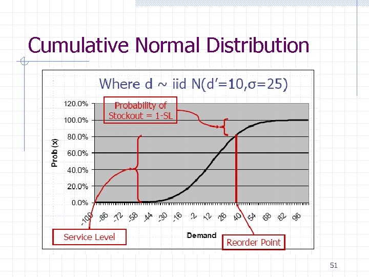Cumulative Normal Distribution 51

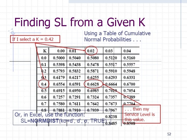Finding SL from a Given K 52

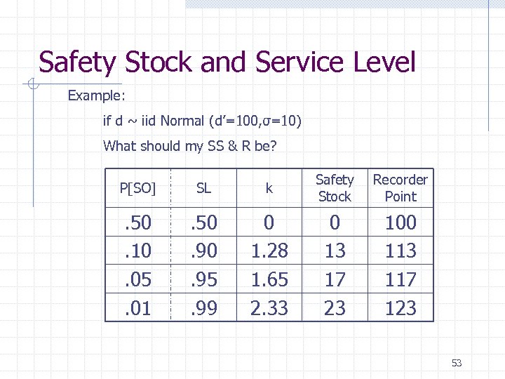Safety Stock and Service Level Example: if d ~ iid Normal (d’=100, σ=10) What should my SS & R be? P[SO] SL k Safety Stock Recorder Point . 50. 10. 05. 01 . 50. 95. 99 0 1. 28 1. 65 2. 33 0 13 17 23 100 113 117 123 53

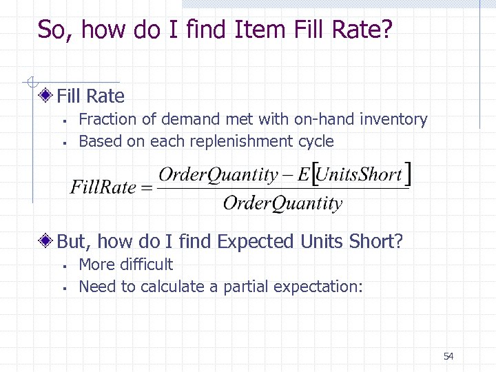So, how do I find Item Fill Rate? Fill Rate § § Fraction of demand met with on-hand inventory Based on each replenishment cycle But, how do I find Expected Units Short? § § More difficult Need to calculate a partial expectation: 54

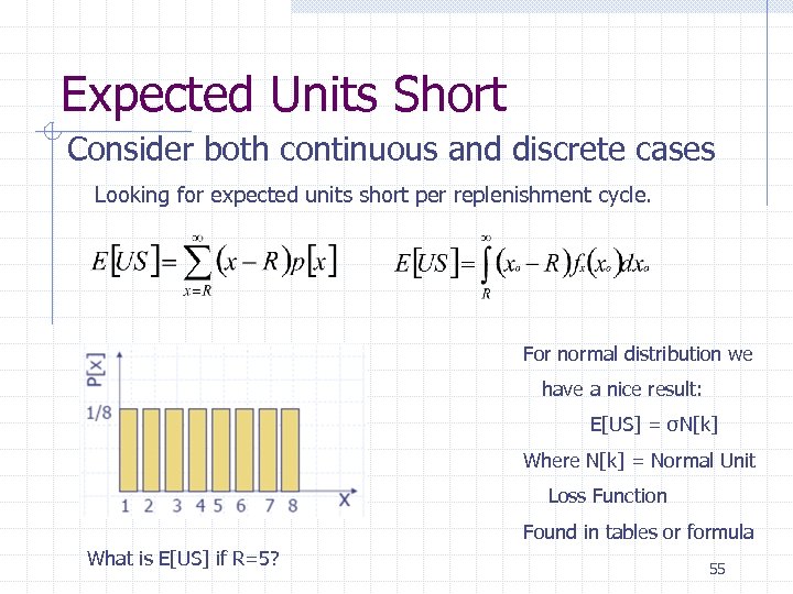Expected Units Short Consider both continuous and discrete cases Looking for expected units short per replenishment cycle. For normal distribution we have a nice result: E[US] = σN[k] Where N[k] = Normal Unit Loss Function Found in tables or formula What is E[US] if R=5? 55

The N[k] Table A Table of Unit Normal Loss Integrals K . 00 . 01 . 02 . 03 . 04 0. 0 . 3989 . 3940 . 3890 . 3841 . 3793 0. 1 . 3509 . 3464 . 3418 . 3373 . 3328 0. 2 . 3069 . 3027 . 2986 . 2944 . 2904 0. 3 . 2668 . 2630 . 2592 . 2555 . 2518 0. 4 . 2304 . 2270 . 2236 . 2203 . 2169 0. 5 . 1978 . 1947 . 1917 . 1887 . 1857 0. 6 . 1687 . 1659 . 1633 . 1606 . 1580 0. 7 . 1429 . 1405 . 1381 . 1358 . 1334 0. 8 . 1202 . 1181 . 1160 . 1140 . 1120 0. 9 . 1004 . 09860 . 09680 . 09503 . 09328 1. 0 . 08332 . 08174 . 08019 . 07866 . 07716 56

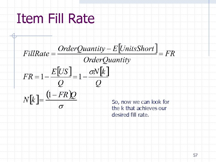Item Fill Rate So, now we can look for the k that achieves our desired fill rate. 57

Finite Horizon Planning 58

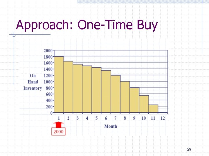Approach: One-Time Buy 59

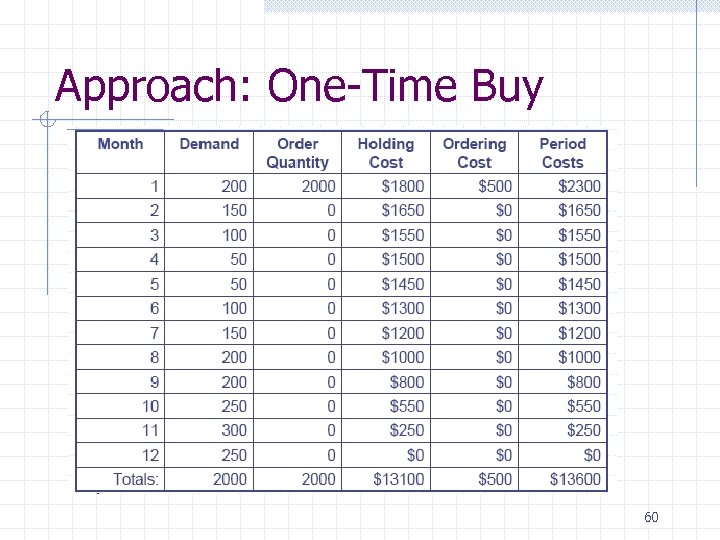Approach: One-Time Buy 60

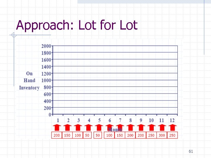Approach: Lot for Lot 61

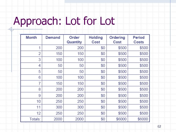Approach: Lot for Lot 62

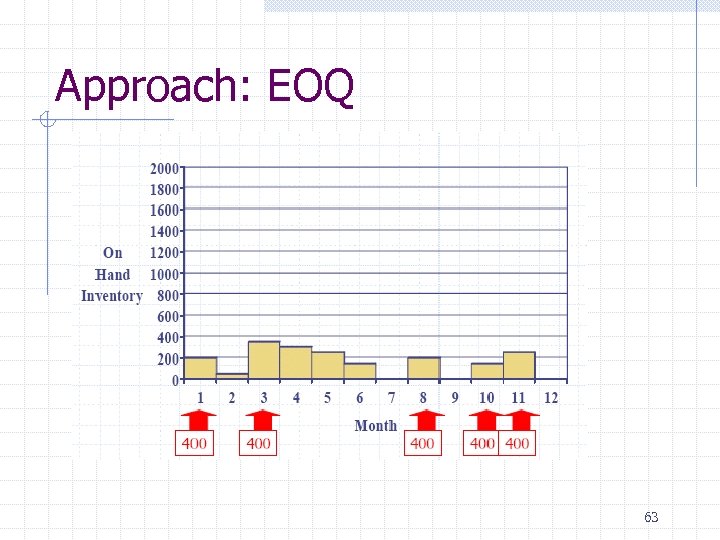Approach: EOQ 63

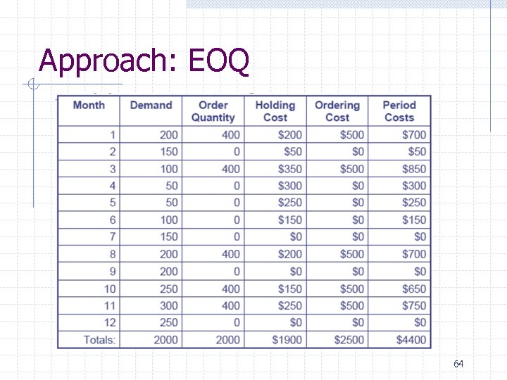Approach: EOQ 64

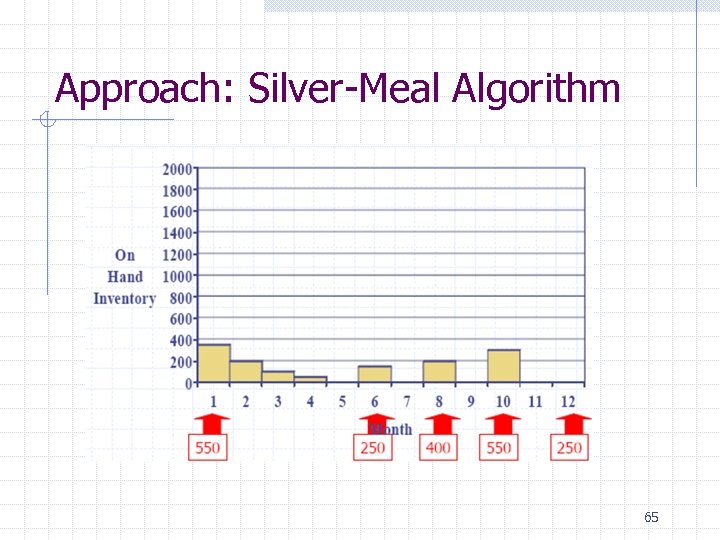Approach: Silver-Meal Algorithm 65

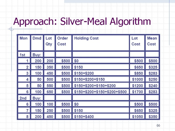Approach: Silver-Meal Algorithm 66

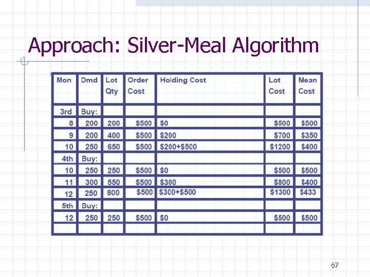Approach: Silver-Meal Algorithm 67

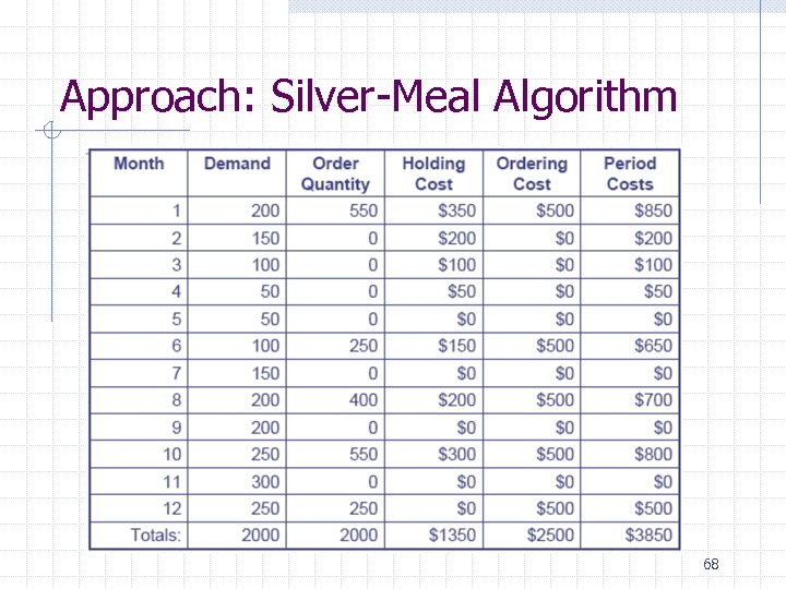Approach: Silver-Meal Algorithm 68

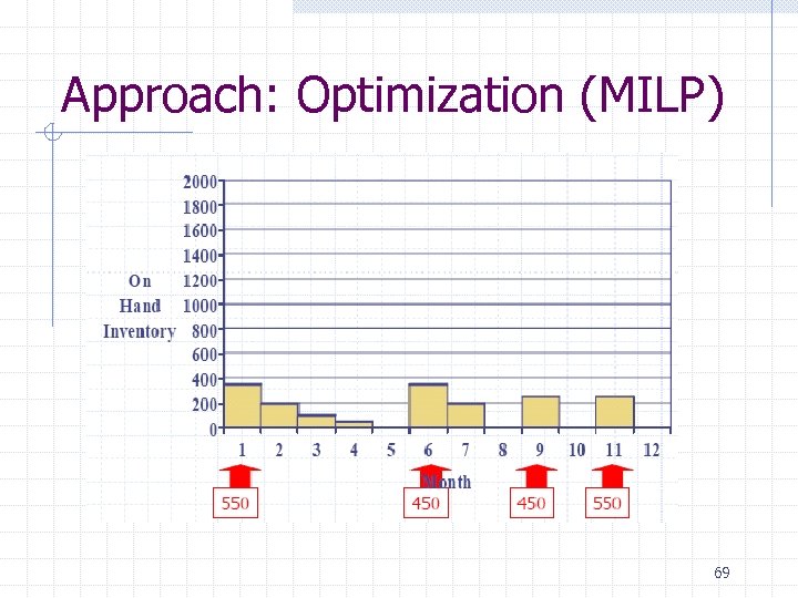Approach: Optimization (MILP) 69

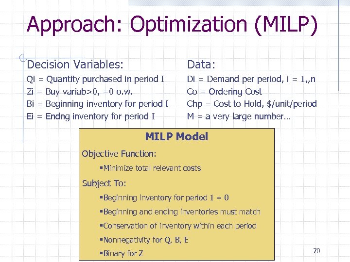Approach: Optimization (MILP) Decision Variables: Data: Qi = Quantity purchased in period I Zi = Buy variab>0, =0 o. w. Bi = Beginning inventory for period I Ei = Endng inventory for period I Di = Demand period, i = 1, , n Co = Ordering Cost Chp = Cost to Hold, $/unit/period M = a very large number… MILP Model Objective Function: §Minimize total relevant costs Subject To: §Beginning inventory for period 1 = 0 §Beginning and ending inventories must match §Conservation of inventory within each period §Nonnegativity for Q, B, E §Binary for Z 70

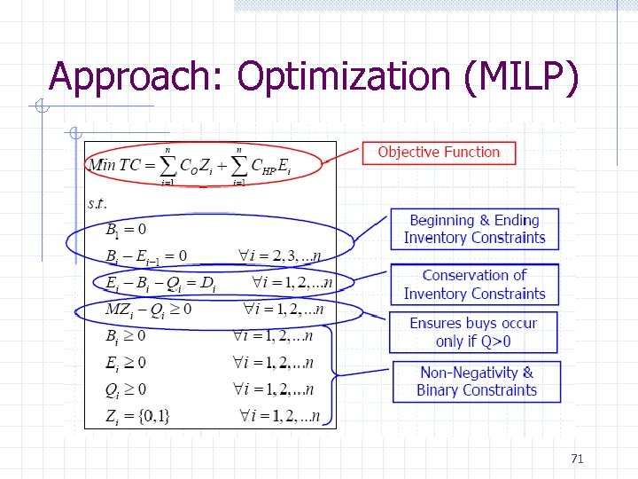Approach: Optimization (MILP) 71

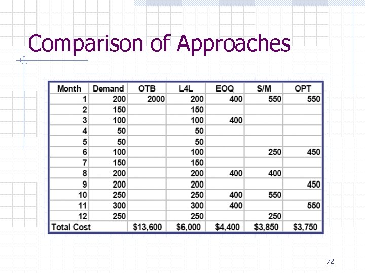Comparison of Approaches 72

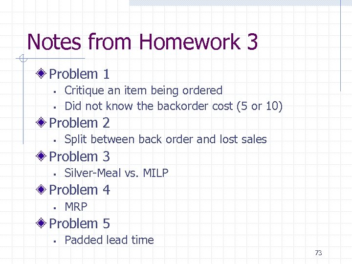Notes from Homework 3 Problem 1 § § Critique an item being ordered Did not know the backorder cost (5 or 10) Problem 2 § Split between back order and lost sales Problem 3 § Silver-Meal vs. MILP Problem 4 § MRP Problem 5 § Padded lead time 73