af8887e9e548163b88c8dd07956694e4.ppt
- Количество слайдов: 85

Revenue Management and Pricing Chapter 3 Basic Price Optimization
Revenue Management and Pricing • The goal of the optimization problem—its objective function—is to maximize contribution: total revenue minus total incremental cost from sales. • The key elements of this problem are the price-response function and the incremental cost of sales. • We formulate and solve the pricing and revenue optimization function in the case of a single product in a single market without supply constraints and derive some important optimality conditions.

Price-Response Function • A fundamental input to any PRO analysis is the price-response function, or price-response curve, d(p) which specifies how demand for a product varies as a function of its price, p. • The price-response function specifies demand for the product of a single seller as a function of the price offered by that seller. This contrasts with the concept of a market demand curve found in economic texts, which specifies how an entire market will respond to changing prices. • The distinction is critical because different firms competing in the same market face different price-response functions. • The differences in the price-response functions faced by different sellers are the result of many factors, such as the effectiveness of their marketing campaigns, perceived customer differences in quality, product differences, and location, among other factors.

Price-Response Function • In a perfectly competitive market, the price response faced by an individual seller is a vertical line at the market price, as shown in Figure 3. 1. • If the seller prices above the market price, his demand drops to 0. If he prices below the market price, his demand is equal to the entire market.

Price-Response Function • In a perfectly competitive market, buyers are totally indifferent among the offerings of different sellers, they have perfect knowledge about all prices being offered, and they will buy the product only from the lowest-price seller. • Furthermore, each seller is small relative to the total size of the market. In this situation, the seller has no pricing decision—his price is set by the operation of the larger market. • At any price below the market price, the demand seen by a seller would be equal to the entire demand in the market. At any price above the market price he sells nothing. • The seller of a true commodity in a perfectly competitive market has no need for pricing and revenue optimization • However, true commodities are surprisingly rare. The vast majority of companies face finite customer responses to price changes and therefore have active PRO decisions.
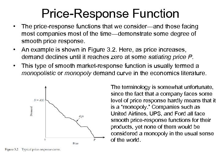
Price-Response Function • The price-response functions that we consider—and those facing most companies most of the time—demonstrate some degree of smooth price response. • An example is shown in Figure 3. 2. Here, as price increases, demand declines until it reaches zero at some satiating price P. • This type of smooth market-response function is usually termed a monopolistic or monopoly demand curve in the economics literature. The terminology is somewhat unfortunate, since the fact that a company faces some level of price response hardly means that it is a “monopoly. ” Companies such as United Airlines, UPS, and Ford all face smooth price-response functions for their products, yet none of them would be considered a monopoly in the usual sense of the world.
Price-Response Function • There are many different ways in which product demand might change in response to changing prices and, thus, many different possible price-response functions. • However, all of the price-response functions we consider will be nonnegative, continuous, differentiable, and downward sloping.

Price-Response Function • Nonnegative: We assume that all prices are greater than or equal to zero; that is, p ≥ 0. • Continuous: We assume that the price-response function is continuous—there are no “gaps” or “jumps” in the market response to our prices. More formally, if d(0)=D and P is the satiating price, that is, the lowest price for which d(P) = 0, then for every 0<q≤D, there is a price p ≤ P such that d(p) = q. This implies that there is a price that will generate any level of demand between 0 and the maximum demand. This property, known as invertability, is often very useful. • Differentiable: Differentiability means that the price-response function is smooth, with a well-defined slope at every point. Differentiability allows us to use the tools of calculus to solve the constrained optimization problems that arise in PRO
Price-Response Function • Downward sloping: We assume that d(p) is downward sloping whenever d(p) > 0— that is, that raising prices for a good during a period will decrease demand for that good during that period unless demand is already 0, in which case demand will remain at 0. • Conversely, lowering prices can only increase demand. • Nonetheless, there at least three cases in which the downwardsloping property may not hold.
Price-Response Function 1. Giffen goods: Economic theory allows for the possibility of socalled Giffen goods, whose demand rises as their price rises because of substitution effects. • An example might be a student on a strict budget of $8. 00 per week for dinner. When hamburger costs $1. 00 per serving and steak costs $2. 00, he eats hamburger six times a week and steak once. If the price of hamburger rises to $1. 10, to stay within his budget, he stops buying steak and buys hamburger seven times a week. In this case, a rise in the price of hamburger causes his consumption of hamburger to increase. • Giffen goods are almost never encountered in reality—in fact, many economists doubt whether they have ever existed.
Price-Response Function 2. Price as an indicator of quality: In some markets, price is used by some consumers as an indicator of quality: Higher prices signal higher quality. In this case, lowering the price for a product may lead consumers to believe that it is of lower quality, and demand could drop as a result. • • Wine is a classic example: Faced with a daunting array of labels and varietals, many purchasers are likely to use a rule such as: a $10 bottle for dinner with the family, a $15 bottle if the couple next door is dropping by, and a $25 bottle if our wine-snob friends are joining us for dinner. The “price-as-an-indicator-of-quality effect” can be particularly important when a new product enters the market. A medical-product company developed a way of producing a home testing device at a cost 75% below the cost of the prevailing technology. They introduced the new product at a list price 60% lower than the list price of the leading competitors, expecting to dominate the market. When sales were slow, they repackaged the product and sold it at a price only 20% lower than the leading competitor. This time sales took off. Their belief is that the initial rock-bottom price induced customers to believe their product was inferior and unreliable. The higher price was high enough not to raise quality concerns but low enough to drive high sales.

Price-Response Function 3. Conspicuous consumption: The situation in which a consumer makes a purchase decision in order to advertise his ability to spend large amounts. • It probably does not come as a shock that the reason some rock stars drink $300 bottles of Cristal champagne and drive Bentleys is not their finely honed appreciation of fine French champagne and British automotive engineering. • Conspicuous consumption postulates a segment of customers who buy a product simply because it has a high price—and others know it. Dropping the price in this case may cause the product to lose its cachet and decrease demand. While duly noting these three exceptions to downward-sloping demand curves, we will proceed to ignore them. We assume that for almost all items, almost all of the time, raising the price will lower demand lowering the price will increase demand.
Measures of Price Sensitivity • It is often useful to have a simple characterization of the price sensitivity implied by a price-response function at a particular price. • The two most common measures of price sensitivity are the slope and the elasticity of the price-response function. • Slope: The slope of the price-response function measures how demand changes in response to a price change. It is equal to the change in demand divided by the difference in prices, or • By the downward-sloping property, p 1 > p 2 implies that d(p 1)≤d(p 2). This means that slope will always be less than or equal to zero. • Above definition requires two prices to be specified, because the slope of a price-response function will be constant across all prices only if it is linear. However, it is common to specify the slope at a single price, say, p 1, in which case it can be computed as the limit of the above equation as p 2 approaches p 1. That is,

Measures of Price Sensitivity • where d’(p 1) denotes the derivative of the price-response function at p 1. By the differentiability property, we know that this derivative exists. • The downward-sloping property means that the slope will be less than or equal to zero for all prices. • The slope can be used as a local estimator of the change in demand that would result from a small change in price. For small changes in price, we can write • That is, a large (highly negative) slope means that demand is more responsive to price than a smaller (less negative) slope.
Measures of Price Sensitivity Ex: The slope of the price-response function facing a semiconductor manufacturer at the current price of $0. 13 per chip is 1, 000 chips/week per cent. • Estimate the approximate effect of a 2 -cent increase in price on the demand – Decrease of 2000 chips • Estimate the approximate effect of a 3 -cent decrease in price on the demand – Increase of 3000 chips
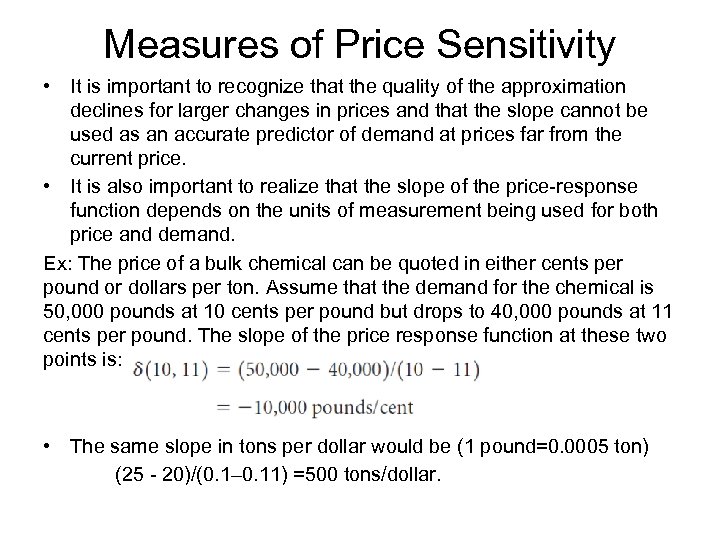
Measures of Price Sensitivity • It is important to recognize that the quality of the approximation declines for larger changes in prices and that the slope cannot be used as an accurate predictor of demand at prices far from the current price. • It is also important to realize that the slope of the price-response function depends on the units of measurement being used for both price and demand. Ex: The price of a bulk chemical can be quoted in either cents per pound or dollars per ton. Assume that the demand for the chemical is 50, 000 pounds at 10 cents per pound but drops to 40, 000 pounds at 11 cents per pound. The slope of the price response function at these two points is: • The same slope in tons per dollar would be (1 pound=0. 0005 ton) (25 - 20)/(0. 1– 0. 11) =500 tons/dollar.
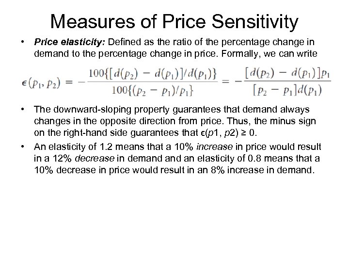
Measures of Price Sensitivity • Price elasticity: Defined as the ratio of the percentage change in demand to the percentage change in price. Formally, we can write • The downward-sloping property guarantees that demand always changes in the opposite direction from price. Thus, the minus sign on the right-hand side guarantees that ϵ(p 1, p 2) ≥ 0. • An elasticity of 1. 2 means that a 10% increase in price would result in a 12% decrease in demand an elasticity of 0. 8 means that a 10% decrease in price would result in an 8% increase in demand.

Measures of Price Sensitivity • ϵ(p 1, p 2) is sometimes called the arc elasticity. That it requires two prices to calculate, reflects that the percentage change in demand resulting from changing prices will depend on both the old price and the new price. • In fact, the percentage decrease in from a 1% increase in price will generally not even be the same as the percentage increase in demand that we would experience from a 1% decrease in price. For this reason, both prices need to be specified in order to fully characterize elasticity. However, as we did with slope, we can derive a point elasticity at p by taking the limit of this equation as p 2 approaches p 1: • In words, the point elasticity is equal to -1 times the slope of the demand curve times the price, divided by demand. • Since d’(p) ≤ 0, the point elasticity ϵ (p) will be greater than or equal to zero. The point elasticity is useful as a local estimate of the change in demand resulting from a small change in price.

Measures of Price Sensitivity Ex: A semiconductor manufacturer is selling 10, 000 chips per month at $0. 13 per chip. He believes that the price elasticity for his chips is 1. 5. Thus, a 15% increase in price from $0. 13 to $0. 15 per chip would lead to • a decrease in demand of about 1. 5 *15% = 22. 5%, or from 10, 000 to about 7, 750 chips per month. • One of the appealing properties of elasticity is that, unlike slope, its value is independent of the units being used. Thus, the elasticity of electricity is the same whether the quantity electricity is measured in kilowatts or megawatts and whether the units are dollars or euros. Ex: Consider the bulk chemical whose price-response slope was estimated before. It showed a 20% decrease in demand (from 50, 000 pounds to 40, 000 pounds) from a 10% increase in price (from 10 cents to 11 cents). The corresponding elasticity is 0. 2/0. 1 = 2—an elastic response. What if the units were euros and tons? It would still be a 20% decrease in demand (from 25 tons to 20 tons) from a 10% increase in price.
Measures of Price Sensitivity • Like slope, point elasticity is a local property of the price-response function. That is, elasticity can be specified between two different prices and a point elasticity defined at a point only gives approximate results. • In practice, the term price elasticity is often used simply as a synonym for price sensitivity. Items with “high price elasticity” have demand that is very sensitive to price while “low price elasticity” items have much lower sensitivity. • Often, a good with a price elasticity greater than 1 is described as elastic, while one with an elasticity less than 1 is described as inelastic.
Measures of Price Sensitivity • Elasticity depends on the time period under consideration, and, as with other aspects of price response, we must be clear to specify the time frame we are talking about. • For most products, short-run elasticity is lower than long-run elasticity. The reason is that buyers have more flexibility to adjust to higher prices in the long run. For example, the short-run elasticity for gasoline has been estimated to be 0. 2, while the long-run elasticity has been estimated at 0. 7. In the short run, the only options consumers have in response to high gas prices are to take fewer trips and to use public transportation. But if gasoline prices stay high, consumers will start buying higher mile-per-gallon cars, depressing overall demand for gasoline even further. • A retailer raising the price of milk by 20 cents may not see much change in milk sales for the first week or so and conclude that the price elasticity of milk is low. But he will likely see a much greater deterioration in demand over time. The reason is that customers who come to shop for milk after the price rise will still buy milk, since it is too much trouble to go to another store. But some customers will note the higher price and switch stores the next time they shop.

Measures of Price Sensitivity • On the other hand, the long-run price elasticity of many durable goods —such as automobiles and washing machines—is lower than the short-run elasticity. • The reason is that customers initially respond to a price rise by postponing the purchase of a new item. However, they will still purchase at some time in the future, so the long-run effect of the price change is less than the short-run effect. • Market elasticity measures total market response if all suppliers of a product increase their prices—perhaps in response to a common cost change. • Market elasticity is generally much lower than the price-response elasticity faced by an individual supplier within the market. The reason is simple: If all suppliers raise their price, the only alternative faced by customers is to purchase a substitute product or to go without. On the other hand, if a single supplier raises its price, its customers have the option of defecting to the competition.

Measures of Price Sensitivity • Table 3. 1 shows some elasticities that have been estimated for various goods and services. • Note that a staple such as salt is very inelastic—customers do not change the amount of salt they purchase very much in response to market price changes. On the other hand, we would expect that price elasticity of the market-response function faced by any individual seller of salt to be quite large—since salt is a fungible commodity in a highly competitive market.
Price Response and Willingness to pay • So far, we have treated the price-response function as simply given. • In reality, demand is the result of thousands, perhaps millions, of individual buying decisions on the part of potential customers. • The price-response function specifies how many more of those potential customers would buy if we lowered our price and how many current buyers would not buy if we raised our price. • We usually cannot directly track the thousands or even millions of individual decisions that ultimately manifest themselves in demand for our product. However, it is worthwhile to understand the assumptions about customer behavior that underlie the price-response functions so that we can judge if the price-response function is based on assumptions appropriate for the application. The most important of such models of customer behavior is based on willingness to pay.
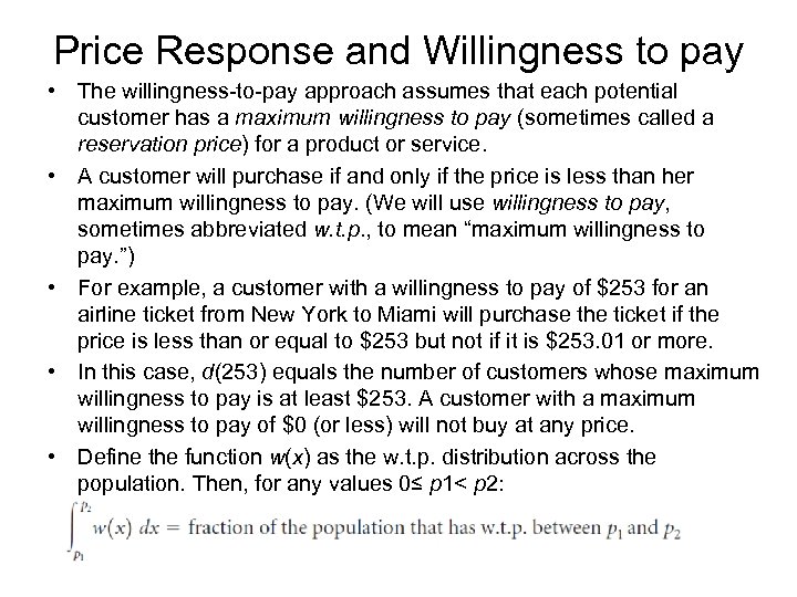
Price Response and Willingness to pay • The willingness-to-pay approach assumes that each potential customer has a maximum willingness to pay (sometimes called a reservation price) for a product or service. • A customer will purchase if and only if the price is less than her maximum willingness to pay. (We will use willingness to pay, sometimes abbreviated w. t. p. , to mean “maximum willingness to pay. ”) • For example, a customer with a willingness to pay of $253 for an airline ticket from New York to Miami will purchase the ticket if the price is less than or equal to $253 but not if it is $253. 01 or more. • In this case, d(253) equals the number of customers whose maximum willingness to pay is at least $253. A customer with a maximum willingness to pay of $0 (or less) will not buy at any price. • Define the function w(x) as the w. t. p. distribution across the population. Then, for any values 0≤ p 1< p 2:

Price Response and Willingness to pay • We note that 0 ≤ w(x) ≤ 1 for all nonnegative values of x. • Let D=d(0), the maximum demand achievable (market size). Then we can derive d(p) from the w. t. p. distribution from • We can take the derivative of the corresponding price-response function to obtain • which is nonpositive, as required by the downward-sloping demand curve property. Conversely, we can derive the willingness-to-pay distribution from the price-response function using
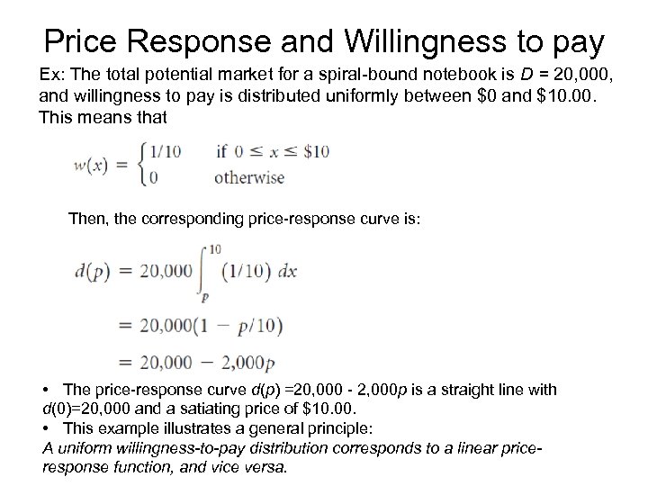
Price Response and Willingness to pay Ex: The total potential market for a spiral-bound notebook is D = 20, 000, and willingness to pay is distributed uniformly between $0 and $10. 00. This means that Then, the corresponding price-response curve is: • The price-response curve d(p) =20, 000 - 2, 000 p is a straight line with d(0)=20, 000 and a satiating price of $10. 00. • This example illustrates a general principle: A uniform willingness-to-pay distribution corresponds to a linear priceresponse function, and vice versa.
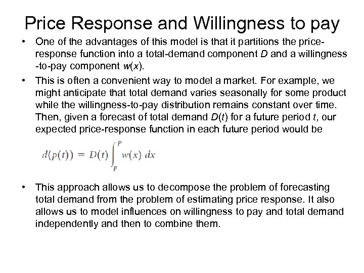
Price Response and Willingness to pay • One of the advantages of this model is that it partitions the priceresponse function into a total-demand component D and a willingness -to-pay component w(x). • This is often a convenient way to model a market. For example, we might anticipate that total demand varies seasonally for some product while the willingness-to-pay distribution remains constant over time. Then, given a forecast of total demand D(t) for a future period t, our expected price-response function in each future period would be • This approach allows us to decompose the problem of forecasting total demand from the problem of estimating price response. It also allows us to model influences on willingness to pay and total demand independently and then to combine them.

Price Response and Willingness to pay • For example, we might anticipate that a targeted advertising campaign will not increase the total population of potential customers, D(t), but that it will shift the willingness-to-pay distribution. • On the other hand, if we open a new retail outlet, we might anticipate that the total demand potential for the new outlet will be determined by the size of the population served, while the willingness to pay will have the same distribution as existing stores serving populations with similar demographics. • Of course, a customer’s willingness to pay changes with changing circumstances and tastes. The maximum willingness to pay for a cold soft drink increases as the weather gets warmer—a fact that the Coca -Cola company considered exploiting with vending machines that changed prices with temperature. (We will discuss “temperaturesensitive vending machine” idea in Chapter 12). • Willingness to pay to see a movie is higher for most people on Friday night than on Tuesday afternoon. • A sudden windfall or a big raise may increase an individual’s maximum willingness to pay for a new Mercedes Benz.

Price Response and Willingness to pay • To the extent that such changes are random and uncorrelated, they will not effect the overall w. t. p. distribution, since increasing willingness to pay on one person’s part will tend to be balanced by another’s decreasing willingness to pay. • On the other hand, systematic changes across a population of customers will change the overall distribution and cause the priceresponse function to shift. Such systematic changes may be due to seasonal effects, changing fashion or fads, or an overall rise in purchasing power for a segment of the population. • These systematic changes need to be understood and incorporated into estimating price response and future price response.

Price Response and Willingness to pay • A disadvantage of the willingness-to-pay formulation is that it assumes that customers are considering only a single purchase. This is a reasonable assumption for relatively expensive and durable items. However, for many inexpensive or nondurable items, a reduction in price might cause some customers to buy multiple units. • A significant price reduction on a washing machine will induce additional customers to buy a new washing machine, but it is unlikely to induce many customers to purchase two. However, a deep discount on socks may well induce customers to buy several pairs. This additional induced demand is not easily incorporated in a willingness-to-pay framework—willingness-to-pay models are most applicable to “big ticket” consumer items and industrial goods.
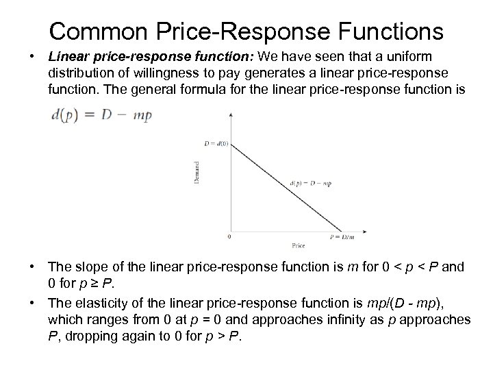
Common Price-Response Functions • Linear price-response function: We have seen that a uniform distribution of willingness to pay generates a linear price-response function. The general formula for the linear price-response function is • The slope of the linear price-response function is m for 0 < p < P and 0 for p ≥ P. • The elasticity of the linear price-response function is mp/(D - mp), which ranges from 0 at p = 0 and approaches infinity as p approaches P, dropping again to 0 for p > P.

Linear price-response function • We will use the linear price-response function in many examples because it is a convenient and easily tractable model of market response. • However, it is not a realistic global representation of price response. • The linear price-response function assumes that the change in demand from a 10 -cent increase in price will be the same, no matter what the base price might be. This is unrealistic, especially when a competitor may be offering a close substitute. In this case, we would usually expect the effect of a price change to be greatest when the base price is close to the competitor’s price.
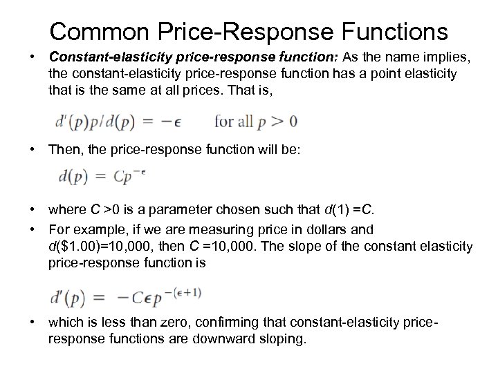
Common Price-Response Functions • Constant-elasticity price-response function: As the name implies, the constant-elasticity price-response function has a point elasticity that is the same at all prices. That is, • Then, the price-response function will be: • where C >0 is a parameter chosen such that d(1) =C. • For example, if we are measuring price in dollars and d($1. 00)=10, 000, then C =10, 000. The slope of the constant elasticity price-response function is • which is less than zero, confirming that constant-elasticity priceresponse functions are downward sloping.

Constant-elasticity price-response function • Note that constant-elasticity price-response functions are neither finite nor satiating. Demand does not drop to zero at any price, no matter how high, and demand continues to approach infinity as price approaches zero. For these reasons, constant elasticity is usually not a good global assumption for price response.

Constant-elasticity price-response function • It is interesting to analyze the impact of price on revenue for a seller facing constant elasticity price response. Let R(p) denote total revenue at price p. Then R(p)=p*d(p) and, for the constant-elasticity price-response function • Taking the slope of this function: • Since d(p) >0, the direction of the slope is determined by the (1 -ϵ) term. If ϵ<1 (that is, if demand is inelastic), then R’(p)>0. This means that the seller facing constant inelastic price response can always increase his revenue by increasing price.

Constant-elasticity price-response function • If ϵ >1, a seller can increase revenue by decreasing price. In fact, the seller can maximize revenue by setting the price as close to zero— without actually becoming zero—as possible! • If ϵ=1, then R(p)=C for any value of p—revenue will not change at all as price changes. • Revenue as a function of price for three different constant-elasticity price-response cases is illustrated in Figure 3. 6.

Constant-elasticity price-response function • These properties make the constant-elasticity function problematic as a global price response function. • It is certainly the rare market in which a seller can maximize his revenue by either increasing his price toward infinity or dropping it as close to zero as possible. • For these reasons, constant elasticity is a better representation of local price response than for use as a global price-response function. • In real-world situations, we would expect price elasticity to change as price changes.
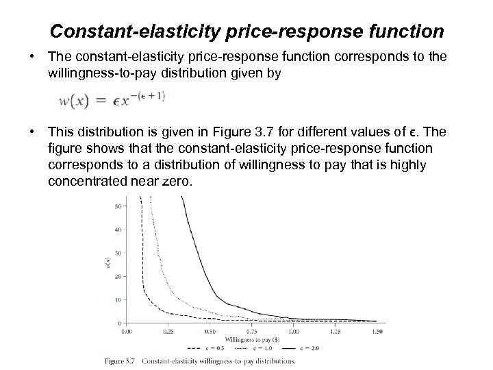
Constant-elasticity price-response function • The constant-elasticity price-response function corresponds to the willingness-to-pay distribution given by • This distribution is given in Figure 3. 7 for different values of ϵ. The figure shows that the constant-elasticity price-response function corresponds to a distribution of willingness to pay that is highly concentrated near zero.

Common Price-Response Functions • The logit price-response functions: Both the linear and the constant-elasticity price response functions have rather severe limitations as global models of customer behavior. • This can be seen by considering their corresponding willingness-topay distributions. The linear price-response function assumes that w. t. p. is uniformly distributed between 0 and some maximum value. The constant-elasticity price-response function assumes that the distribution of willingness to pay drops steadily as price increases, approaching, but never reaching, zero. Neither of these functions would seem to represent customer behavior very realistically. • How would we expect customers to react to changes in price?
The logit price-response function • Consider the case where we are selling a compact car. Assume that competing models are generally similar to ours and are selling at a market price of about $13, 000. If we price well above the market price, say, at $20, 000, we won’t sell many cars. But the few customers who are buying from us at $20, 000 must be very loyal (or very ignorant)—we would not expect to lose very many more of them if we increased our price from $20, 000 to $21, 000. In other words, the elasticity of the price response function is low at this price. • On the other hand, if we priced well below the market price—say, at $9, 000—we would expect to sell lots of cars. At this price, almost anyone who wants to buy a compact car and is not incredibly loyal to another brand (or incredibly averse to ours) would be buying from us. Lowering our price another $1, 000 is unlikely to attract many new customers. Again, price elasticity is low.

The logit price-response function • What happens when we are close to the market price? In this case, we would expect small changes in our price to lead to substantial shifts in demand. There a lot of customers who are more or less indifferent between our offering and that of the competition. Many of these customers can be persuaded to purchase our car if we ask only $250 less than the market price, and even more will shift if we ask $500 less than the market price. Similarly, if we charge $250 above the market price we are likely to lose a lot of demand to the competition. In other words, price elasticity is highest when we are at (or near) the market price.

The logit price-response function • This kind of consumer behavior generates a response curve of the general form shown in Figure 3. 8. When we price very low, we receive lots of demand, but demand changes slowly as we change price. In the area of the “market price, ” demand is very sensitive to our price—small changes in price can lead to substantial changes in demand. At high prices, demand is low and changes slowly as we raise prices further. The price-response curve has a sort of reverse S shape. Empirical research has shown that this general form of price response curve fits observed price response in a wide range of markets.

The logit price-response function • The most popular price-response function of this form is the logit price -response function: • Here, a, b, and C are parameters with C >0 and b >0. a can be either greater than or less than 0, but in most applications we will have a >0. • Broadly speaking, C indicates the size of the overall market and b specifies price sensitivity. Larger values of b correspond to greater price sensitivity. The price-sensitivity curve is steepest at the point p=-(a/b), as indicated in Figure 3. 8. This point can be considered to be approximately the “market price. ”
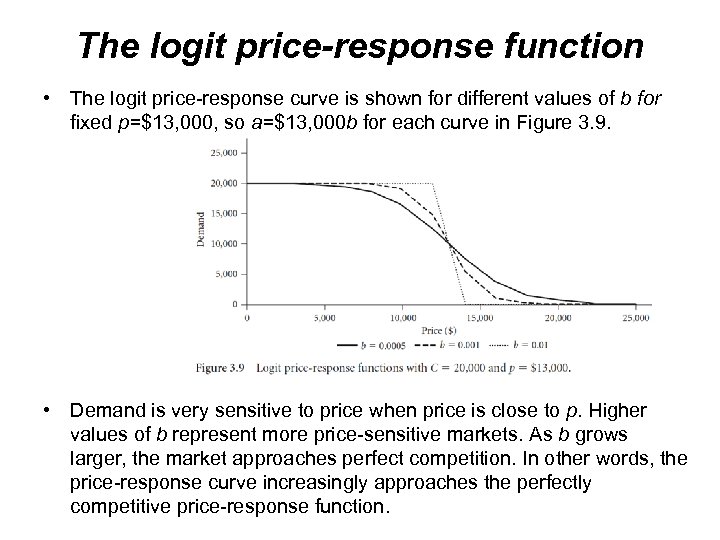
The logit price-response function • The logit price-response curve is shown for different values of b for fixed p=$13, 000, so a=$13, 000 b for each curve in Figure 3. 9. • Demand is very sensitive to price when price is close to p. Higher values of b represent more price-sensitive markets. As b grows larger, the market approaches perfect competition. In other words, the price-response curve increasingly approaches the perfectly competitive price-response function.
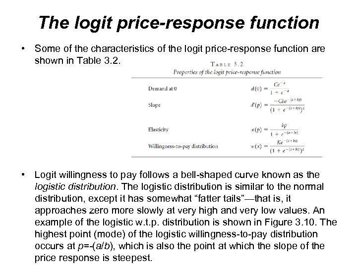
The logit price-response function • Some of the characteristics of the logit price-response function are shown in Table 3. 2. • Logit willingness to pay follows a bell-shaped curve known as the logistic distribution. The logistic distribution is similar to the normal distribution, except it has somewhat “fatter tails”—that is, it approaches zero more slowly at very high and very low values. An example of the logistic w. t. p. distribution is shown in Figure 3. 10. The highest point (mode) of the logistic willingness-to-pay distribution occurs at p=-(a/b), which is also the point at which the slope of the price response is steepest.

The logit price-response function • This is a far more realistic w. t. p. distribution than those associated with either the constant-elasticity or linear price-response functions. • For that reason, the logit is usually preferred to linear or constantelasticity price-response functions when the effects of large price changes are being considered.

Price-response with competition • So far we have not given much attention to the issue of competition. • We have mentioned a “market price” as the steepest point in the logit price-response function, but we have not made an explicit link with competition. • Yet competition is an important—some may say the most important— fact of life in any market of interest. Most managers identify competition as the number-one factor influencing their pricing. Many complain about being at the mercy of their competitors who have “stupid” or “irrational” pricing. • How should we factor competition into our calculation of price response? • There are three different levels at which competition might be included in PRO. In increasing levels of sophistication and difficulty they are: incorporating competition in the price-response function, explicitly modeling consumer choice, and trying to anticipate competitive reaction.

Incorporating Competition in the Price. Response Function • In many cases, competitive prices may not be available at the time prices need to be optimized. This is especially true in business-tobusiness markets, when the pocket price of the customer may include discounts that are never made visible to the competition. • But it is also true in many consumer markets. Retailers generally have a good idea of what their major competitors are charging at any particular time, but they usually don’t have the time or resources to do exhaustive research on a daily or weekly basis. • Is there any hope of optimizing prices if we don’t know what the competition is doing? • The answer is yes. First of all, the price-response function we will be using in a market will be based on history. To this extent, it already includes “typical” competitive pricing. (Indeed, it would be difficult, if not impossible, to estimate a price-response function that did not include competition. )

Incorporating Competition in the Price. Response Function • To the extent that our competitors will behave in a similar fashion in the future as they have in the past, the price-response function will be a fair representation of market response—including competitive response. • What if the market has changed? • Then, in part, we must rely on the “fast-feedback loop” in the PRO process. If we have a competitor who responds more aggressively to a price action than in the past, this will be manifested in the demand we see in the next period. We have the opportunity to adjust our price -response function and re-optimize accordingly.

Consumer-Choice Modeling • Of course, if we have access to current competitive prices, we should be able to use that information to help us better predict customer response to our own price. This information is increasingly available, particularly for online markets. • For example, the Online Petroleum Information System (OPIS) posts a daily list of prices for different grades of petroleum products offered by different sellers in all major markets in the United States and Canada. • Consumer-choice modeling is based on the situation in which a number of competitors are providing similar products or services to some population of customers.

Consumer-Choice Modeling • Each of the competitors sets a price for the product. Each customer has a vector of willingnesses to pay (or reservation prices), one for each product. • These different w. t. p. ’s represent the different values that she places on the features and “brand value” associated with each product—a more desirable product will have a higher associated w. t. p. • The surplus for each customer and each product is defined as the difference between the customer’s willingness to pay and the price of each product. • Each customer purchases the product with the highest positive surplus. If none of the products has a positive surplus for a customer, she will not purchase at all.

Consumer-Choice Modeling Ex: A customer is shopping for stereo amplifiers at the local Stereo Hut store. Stereo Hut sells five amplifiers at the following prices: • This customer would purchase the Koshiba amplifier since it provides her with the highest surplus. • Note that, in the example, the customer does not buy either the cheapest alternative (Audio Two) or his favorite alternative (Cacophonia). Rather, she purchases the alternative that yields the highest surplus.

Consumer-Choice Modeling • We would expect that each customer would have a different set of reservation prices based on the value she places on the various features of each alternative or her preference for a particular brand. • As before, we can imagine that the reservation prices would be distributed across the population in an n-dimensional bell-shaped curve. • Assume now we have a fixed population of potential buyers and that each of these buyers has positive surplus for at least one of the alternatives. Then, the market share that will be obtained by a particular alternative is:
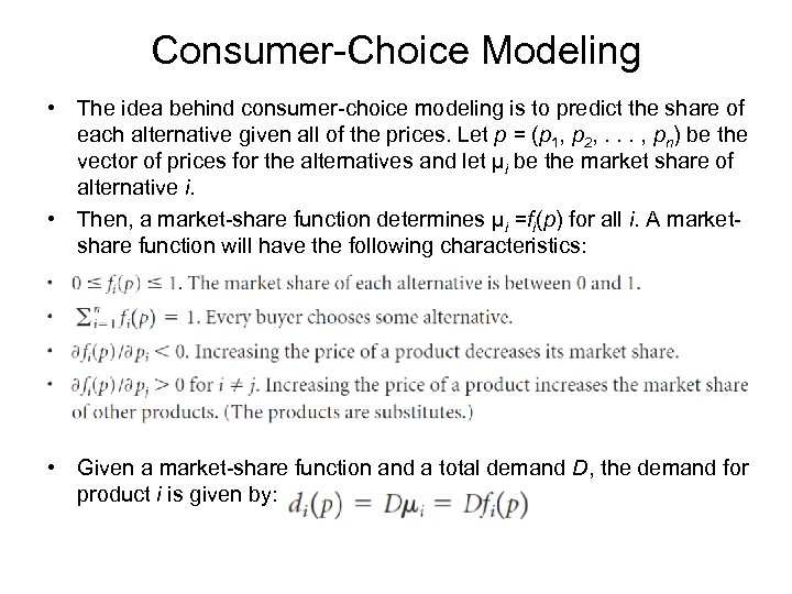
Consumer-Choice Modeling • The idea behind consumer-choice modeling is to predict the share of each alternative given all of the prices. Let p = (p 1, p 2, . . . , pn) be the vector of prices for the alternatives and let µi be the market share of alternative i. • Then, a market-share function determines µi =fi(p) for all i. A marketshare function will have the following characteristics: • Given a market-share function and a total demand D, the demand for product i is given by:
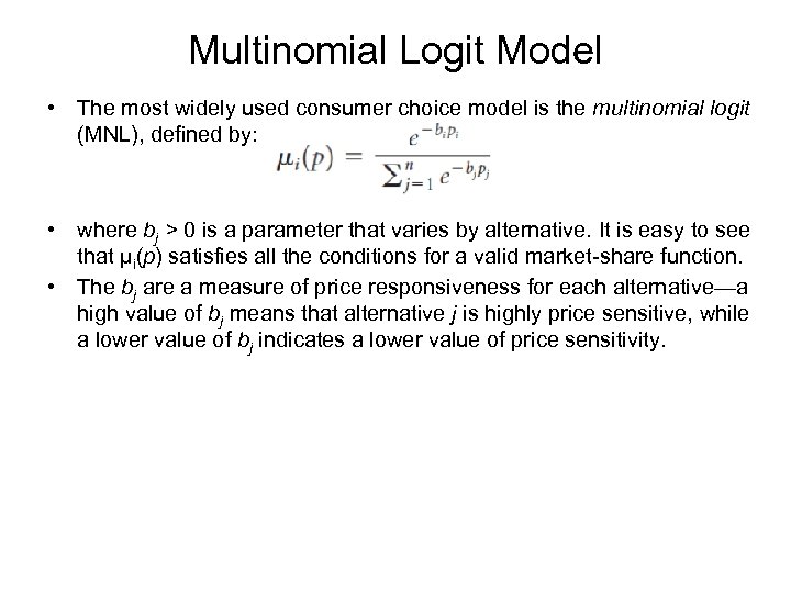
Multinomial Logit Model • The most widely used consumer choice model is the multinomial logit (MNL), defined by: • where bj > 0 is a parameter that varies by alternative. It is easy to see that µi(p) satisfies all the conditions for a valid market-share function. • The bj are a measure of price responsiveness for each alternative—a high value of bj means that alternative j is highly price sensitive, while a lower value of bj indicates a lower value of price sensitivity.
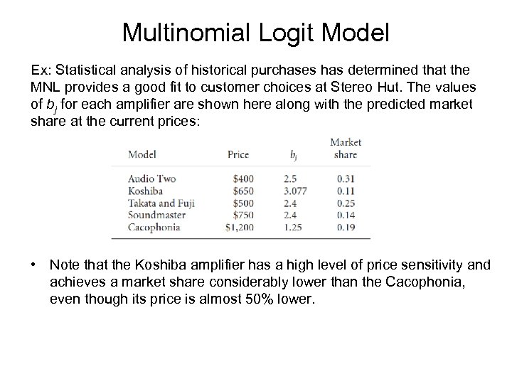
Multinomial Logit Model Ex: Statistical analysis of historical purchases has determined that the MNL provides a good fit to customer choices at Stereo Hut. The values of bj for each amplifier are shown here along with the predicted market share at the current prices: • Note that the Koshiba amplifier has a high level of price sensitivity and achieves a market share considerably lower than the Cacophonia, even though its price is almost 50% lower.

Multinomial Logit Model • In the case where competitive prices are constant, the MNL reduces to the logit price-response function. To see this, assume that prices p 2, p 3, . . . , pn are held constant. Then we can replace the competitive -price term with a constant. That is, we can set • where we have set a = ln(K) and we use the fact that ln(1/K)=-ln(K). • This is the same as the logit price-response function. If we anticipate that competitive prices will be largely stable, the MNL provides little or no additional predictive value over a logit price-response function.

Consumer-Choice Modeling • There a number of weaknesses to consumer-choice modeling as well. One is that, the models assume that all customers purchase some alternative. However, it may be that some customers choose not to purchase at all, since their willingness to pay for every alternative may be below the price of that alternative. Thus, the estimation of the total market D is not really independent of the prices being offered. Indeed, it seems intuitive that an aggressive discount by one supplier would not only siphon customers away from competitors but actually induce customers into the market who might not have purchased from any alternative. • Another drawback of the consumer-choice modeling approach is that, in theory, it requires information on all competitive prices. However, in most markets, companies typically identify two to five companies they consider important competitors. In these cases, one commonly used approach is to derive a competitive index price by weighting the prices offered by the major competitors and using this index as a single competitive price in a multinomial logit.
Anticipating Competitive Response • Even extensive consumer-choice modeling does not provide perfect results. After all, if we are taking competitive prices into account in setting our prices, we should anticipate that our competitors will take our price into account when they set their prices. If we drop a price, we should anticipate the possibility that competitors will match, possibly erasing much of the additional demand we might otherwise predict. The results of raising a price would certainly be different depending upon whether or not our competitors decided to match. • Attempts to predict competitive response and incorporate it into current pricing decisions falls within the realm of decision analysis, or game theory.
Anticipating Competitive Response • The philosophy of pricing and revenue optimization is to make money by many small adjustments, searching for and vacuuming up small and transient puddles of profit as they appear in the marketplace. It is about making a little more money from each transaction. It is not about finding the great pricing move that will stagger the competition with one blow. • Many of the price adjustments called for by pricing and revenue optimization are likely to fall below the radar screen of the competition and may not trigger any explicit response whatsoever. • This does not mean that competitive response need never be considered in pricing. The potential competitive responses to major “bet-the-company” bids or substantial changes in pricing strategy need to be carefully considered.

Anticipating Competitive Response • For example, in the early 1990 s, Hertz Rent-a-Car initiated the use of a sophisticated pricing optimization system. Previously, Hertz, like other national rent-a-car companies, had changed prices only rarely. • Whenever one of the rental car companies dropped a price, the others were likely to follow immediately—often with even larger drops —precipitating an industrywide fare war. • Hertz took great pains to communicate to the industry that its new system would be changing prices much more commonly than before —some prices would go up, some would go down, but all would change much more frequently. The communication was successful: Hertz was able to initiate its revenue management program without inciting retaliatory price wars. • Once Hertz initiated revenue management, it was able to generate additional revenue through thousands of small adjustments to prices that its competitors were unable to match.
Incremental Costs • Costing seems like it should be the easy part of pricing and revenue optimization. After all, a company may not know the price-response function it faces, but surely it should know its own costs. • Unfortunately, things are not quite so simple. With any exposure to the field of accounting one will quickly realize that the simple question “How much did this product cost? ” usually does not have a simple answer. Rather, the “cost” of producing even a simple product depends on who wants to know and what they are going to use the answer for. • Accountants have derived a host of product-costing methodologies, including fully allocated costs, partially allocated costs, marginal costs, avoided costs, and financial costs, to name just a few. • While each costing methodology has its place, pricing and revenue optimization decisions are based on the incremental cost of a customer commitment, where incremental cost is defined as follows. – The incremental cost of a customer commitment is the difference between the total costs a company would experience if it makes the commitment and the total cost it would experience if it doesn’t.
Incremental Costs Calculating incremental cost for a customer commitment depends critically on the context and nature of the commitment. Here are some examples: • An airline is considering whether or not to sell a single seat to a passenger on a future flight. The incremental cost is the additional meal and fuel cost that would be incurred from flying an additional passenger plus any commissions or fees the airline would pay for the booking. • A retailer buys a stock of fashion goods at the beginning of the season. Once he has bought the goods, he cannot return them and cannot reorder. During the season he wants to set and update the prices that will maximize the total revenue he will receive from the fashion goods. Since the cost of the goods is sunk and selling a unit will not drive any additional future sales, his incremental cost per sale is zero. • A drugstore sells bottles of shampoo and replenishes its stock weekly. Because selling a unit will result in an additional unit order, the incremental cost for selling a bottle of shampoo is the wholesale unit cost.
Incremental Costs • A distributor is bidding for a year-long contract with a hospital to be the preferred provider for disposable medical supplies. From previous experience, the distributor knows that this hospital is an expensive customer requiring high levels of customer support, wide variances in orders, and high rates of product returns. The expected incremental cost of the contract includes not only the expected cost of the items the hospital will purchase, but also the expected cost of customer service, operating costs and holding costs driven by the wide variance in orders, and the expected costs of returns. These examples illustrate some of the key characteristics of incremental cost. These characteristics can be summarized as follows. • Incremental cost is forward looking: It is based on the effect a customer commitment will have on future costs. Costs that have already been taken or that are driven by decisions already made prior to the customer commitment are sunk and do not enter into the calculation of incremental cost.
Incremental Costs • Incremental cost is marginal: It is the expected cost of making this customer commitment. The incremental cost of making this commitment may not be the same as the average cost of similar commitments made in the past. • Incremental cost is not fully allocated cost: Only costs that change as the result of a customer commitment are part of the incremental cost. Overhead, or fixed costs of staying in business, may not be allocated to any specific commitment. As a result, the incremental cost of a customer commitment is usually less than the fully allocated cost. Further, the sum of the incremental costs of all commitments will be less than the total operating cost of the company, since there will remain an unallocated residual fixed cost after all the incremental costs have been totaled. • The elements of incremental cost can depend on the type, size, and duration of the commitment: Specifically, if the customer commitment is a multiunit order, then order-based or setup costs need to be allocated across all the units in the order.

Incremental Costs • The incremental cost of a commitment can be uncertain: Trucking companies sell contracts to shippers. Each contract covers the next year and commits the trucking company to carry all the freight tendered by the customer at an agreedon tariff. – The incremental cost associated with one of these contracts is likely to be highly uncertain at the time the commitment is made. – The amount, timing, and origin and destination of the freight the customer will tender over the next year is uncertain. – In addition, the cost of moving the customer’s freight will depend on the freight the company will move for other customers, which is also uncertain. – This cost will depend in part on what portion of the customer’s freight is backhaul business, which can utilize excess capacity on existing trucks, and what portion will be headhaul freight, which will require running new trucks.

Basic Price Optimization • The difference between the price at which a product is sold and its incremental cost is called its unit margin or just margin. • The sum of the margins of all products sold during a time period is called the total contribution. • In most cases, the seller’s goal is to maximize total contribution. • When the supplier is selling a single product at a single price, her total contribution will be: • where m(p) is total contribution and c is incremental cost. The basic price optimization problem is:
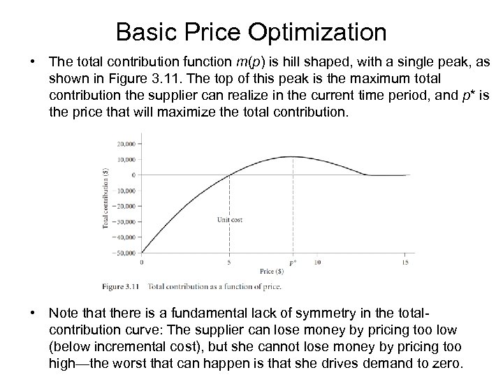
Basic Price Optimization • The total contribution function m(p) is hill shaped, with a single peak, as shown in Figure 3. 11. The top of this peak is the maximum total contribution the supplier can realize in the current time period, and p* is the price that will maximize the total contribution. • Note that there is a fundamental lack of symmetry in the totalcontribution curve: The supplier can lose money by pricing too low (below incremental cost), but she cannot lose money by pricing too high—the worst that can happen is that she drives demand to zero.

Basic Price Optimization • This problem is an unconstrained optimization problem, and standard optimization theory tells us that it can be solved by taking the derivative of m(p) and setting it equal to zero. The derivative of m(p) with respect to price is given by: • To find the price that maximizes total contribution, we set m’(p)=0, or • Thus, a p* satisfying contribution. will maximize total

Basic Price Optimization • Marginal revenue equals marginal cost: When we rewrite the optimality equation: • The term on the left-hand side is marginal revenue—the derivative of total revenue with respect to price. This is the amount of additional revenue the seller could achieve from a small increase in price. Typically, marginal revenue is greater than zero at low prices but less than zero at higher prices. When price is low, increasing price leads to increased total revenue because the reduced demand is outweighed by increased margin. But at some price, the effect of raising price further is to decrease total revenue as demand begins to drop more quickly than margin increases. • The term on the right-hand side is marginal cost: the amount of additional cost the seller would incur from a small increase in price. Note that marginal cost is always less than or equal to zero—an increase in price results in lower demand (by the downward-sloping property), which in turn leads to lower total costs. • This equation states that contribution is maximized when marginal revenue equals marginal cost.
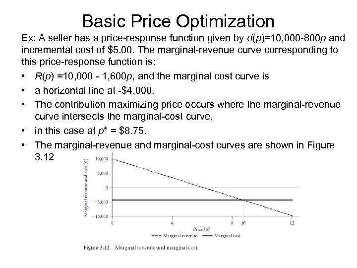
Basic Price Optimization Ex: A seller has a price-response function given by d(p)=10, 000 -800 p and incremental cost of $5. 00. The marginal-revenue curve corresponding to this price-response function is: • R(p) =10, 000 - 1, 600 p, and the marginal cost curve is • a horizontal line at -$4, 000. • The contribution maximizing price occurs where the marginal-revenue curve intersects the marginal-cost curve, • in this case at p* = $8. 75. • The marginal-revenue and marginal-cost curves are shown in Figure 3. 12

Basic Price Optimization We can state this important condition as follows: • Total contribution is maximized in the basic price optimization problem at the price at which marginal revenue equals marginal cost. • Optimality equation provides further useful guidance on price changes that could improve total contribution. If marginal revenue is greater than marginal cost, then the supplier can increase his contribution by increasing price. If, on the other hand, marginal revenue is lower than marginal cost, he should decrease his price to increase contribution.

Basic Price Optimization • Optimal contribution margin and elasticity: We can also relate the optimal price to point elasticity. • where ϵ(p) is point elasticity. • The second term, -d’(p)c, will always be greater than or equal to zero since d’(p)≤ 0. If d(p) >0, then m(p) will always be greater than zero if ϵ(p)<1. In other words, – If the point elasticity at our current price is less than 1, we can increase total contribution by increasing price.
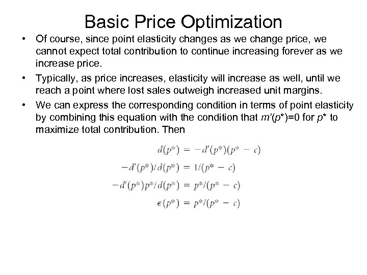
Basic Price Optimization • Of course, since point elasticity changes as we change price, we cannot expect total contribution to continue increasing forever as we increase price. • Typically, as price increases, elasticity will increase as well, until we reach a point where lost sales outweigh increased unit margins. • We can express the corresponding condition in terms of point elasticity by combining this equation with the condition that m’(p*)=0 for p* to maximize total contribution. Then
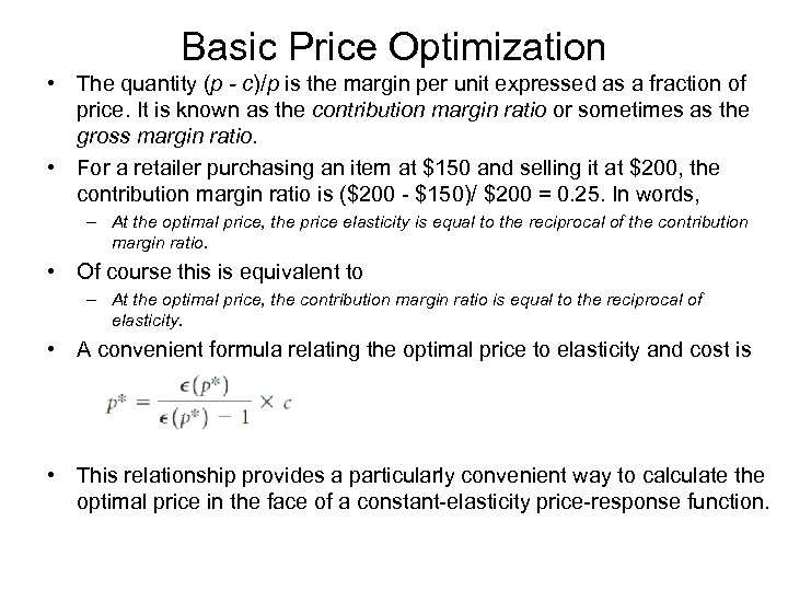
Basic Price Optimization • The quantity (p - c)/p is the margin per unit expressed as a fraction of price. It is known as the contribution margin ratio or sometimes as the gross margin ratio. • For a retailer purchasing an item at $150 and selling it at $200, the contribution margin ratio is ($200 - $150)/ $200 = 0. 25. In words, – At the optimal price, the price elasticity is equal to the reciprocal of the contribution margin ratio. • Of course this is equivalent to – At the optimal price, the contribution margin ratio is equal to the reciprocal of elasticity. • A convenient formula relating the optimal price to elasticity and cost is • This relationship provides a particularly convenient way to calculate the optimal price in the face of a constant-elasticity price-response function.
Basic Price Optimization Ex: An electronics goods retailer faces a constant-elasticity priceresponse function with an elasticity of 2. 5 for a popular model of television. It costs him $180 a piece to purchase the televisions wholesale. At the optimum price, he should achieve a contribution margin ratio of • 1/2. 5 = 40% per unit. This means he should price the televisions at • (2. 5/1. 5) * $180 = $300 in order to maximize total contribution. Imputed price elasticity: We can derive local price elasticity in a market from the contribution margin at the optimal price. Ex: A seller believes he is pricing optimally, and his contribution margin ratio is 20%. This can only be true if the price elasticity is 5. Imputed price elasticity is a good “reality check” on the credibility of a company’s current pricing.

Basic Price Optimization Ex: A widget maker is looking to set the price of widgets for the current month. Assume that the widget maker’s unit production cost c is a constant $5. 00 per widget and that his demand for the current month is governed by the linear price-response function. This means that the demand for widgets will be: d(p)=[10, 000 - 800 p]+ This means that demand will be 10000 -800 p for prices between zero and $12. 50 and that the demand will be 0 for prices over $12. 50. • In this simple example, d’(p) = 800. We can see that the optimal price p* must solve $10, 000 - 800 p* = 800(p* - $5. 00) • or, after a little algebra, 1600 p*=14000 or p*=8. 75. At the optimal price of $8. 75, total widget sales will be 10, 000 -800($8. 75) =3, 000 units, total revenue will be 3, 000*$8. 75=$26, 250, and total contribution will be 3, 000($8. 75 -$5. 00), or $11, 250. Note that total contribution is zero at p=c=$5. 00, rises to a maximum at p*=$8. 75, and drops to zero again at p=$12. 50.

Marginality Test • • One way to check the optimality of p* is to use the marginality test, which states that a particular price can only be optimal if raising the price by a penny or lowering the price by a penny results in reduced margin contribution. The principle of marginality should be pretty obvious—if we could increase contribution by changing the price, then the current price would not be optimal —but it is a useful check nonetheless. Table 3. 3 shows the results of varying the price in this example from $8. 74 to $8. 76. As expected, the price of $8. 75 results in the highest margin of the three alternatives. However, the pattern of change among the prices is instructive: At $8. 74 we are selling eight more units per month, but this is not enough to make up for the lost margin per unit. At $8. 76 we are making a penny more per unit sold, but this is offset by the loss of sales of eight units. The optimal price is $8. 75.

Maximizing Revenue • In some cases, a company might wish to maximize total revenue (rather than total contribution). In this case, the objective function will be: • It is easy to see that this is equivalent to the previous problem when c=0. A company with incremental cost of zero can maximize net contribution by maximizing revenue. • There are some service industries, such as movie theaters, video rentals, and sporting events, in which the incremental costs are close to zero. • Also, incremental costs are zero (or very small) in many cases in which a company has already purchased a fixed amount of perishable, nonreplenishable inventory. This is the situation faced by many fashiongoods retailers, who purchase inventory for an entire season ahead of time. Once the inventory has been purchased, the incremental cost of a sale is zero—and the seller should set prices accordingly. Many of these situations count as markdown opportunities.

Maximizing Revenue • The revenue-maximizing price, p, can be found by differentiating R(p) and setting the derivative equal to 0. Specifically, • In other words, the revenue-maximizing price occurs where the elasticity of the price-response function is equal to 1. • This implies that there is no unconstrained revenue maximizing price associated with a constant-elasticity price-response function unless the price elasticity happens to be exactly 1—in which case, revenue is constant at all prices. • Contribution is maximized when marginal revenue is equal to marginal cost. • Contribution is maximized when marginal revenue is equal to zero.

Maximizing Revenue • Typically, marginal revenue is a decreasing function of price (at least in the region of the optimal price). In this case, we can show marginal revenue and marginal cost can be used to compute the revenue-maximizing and contribution-maximizing prices in Figure 3. 14. • Specifically, we can see that, as long as the marginal revenue curve is decreasing, the revenue-maximizing price is lower than the contribution -maximizing price.

Maximizing Revenue Ex: The CEO of the widget-making company decides that the firm’s goal for the next month will be to maximize revenue from widget sales as part of the long-term strategy to increase market share. The resulting revenuemaximizing price is • equal to $6. 25, with corresponding sales of 5, 000 units. • The corresponding per unit margin is $1. 25, and the total contribution margin is 5, 000*$1. 25=$6, 250. • We can compare this to the maximum margin contribution of $11, 250 and conclude that to maximize total revenue, the company needs to give up $11, 250 - $6, 250=$5, 000 of contribution margin. • The decision that management needs to make in this example is whether or not it is worth giving up a total contribution of $5, 000 per month to “buy” an additional 2, 000 units of demand. Since the revenuemaximizing price is lower than the contribution-maximizing price, there is no guarantee that the revenue-maximizing price will provide a reasonable margin—or even a positive margin—if incremental cost is greater than zero. For this reason, it is dangerous to maximize total revenue without including a constraint that ensures that the resulting price is greater than incremental cost.

Weighted Combinations of Revenue and Contribution • In some cases, a company might wish to maximize a weighted combination of total contribution and revenue. • Some pricing and revenue optimization systems use “slider bars” to determine how much to weight revenue relative to contribution. • The most common approach to combining revenue contribution is to use a weighting parameter α, with 0 ≤ α ≤ 1, resulting in a weighted objective function Z(p) given by • For α=1, Z(p) equals total contribution; for α=0, Z(p) equals revenue. • Values of α between 0 and 1 will maximize a weighted combination of the two, with higher values of α resulting in a higher weighting for contribution relative to total revenue. After some algebra
Weighted Combinations of Revenue and Contribution • This shows that maximizing a weighted combination of the revenue and total contribution is the same as maximizing contribution with a discounted cost. • For example, a value of α=0. 5 implies equal weights for total revenue and total contribution. • The price that maximizes this weighted objective function can be found by maximizing total contribution with cost reduced by 50%. • The price that maximizes a weighted combination of revenue and contribution is greater than or equal to the revenue-maximizing price and less than or equal to the contribution-maximizing price. • In the absence of other constraints, we would only be interested in prices greater than the revenue-maximizing price and less than the contribution-maximizing price. In other words, there is no reason for an unconstrained seller to consider pricing outside of this range.
af8887e9e548163b88c8dd07956694e4.ppt