Returns and Expected Returns 1 Holding period return

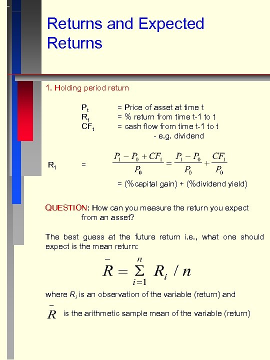Returns and Expected Returns 1. Holding period return Pt Rt CFt R 1 = Price of asset at time t = % return from time t-1 to t = cash flow from time t-1 to t - e. g. dividend = = (%capital gain) + (%dividend yield) QUESTION: How can you measure the return you expect from an asset? The best guess at the future return i. e. , what one should expect is the mean return: where Ri is an observation of the variable (return) and is the arithmetic sample mean of the variable (return)

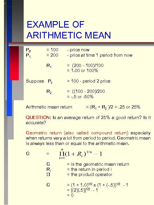EXAMPLE OF ARITHMETIC MEAN P 0 P 1 = 100 = 200 - price now - price at time 1 period from now R 1 = (200 - 100)/100 = 1. 00 or 100% Suppose P 2 R 2 = 100 - period 2 price = ((100 - 200)/200 = -. 5 or -50% Arithmetic mean return = (R 1 + R 2 )/2 =. 25 or 25% QUESTION: Is an average return of 25% a good return? Is it accurate? Geometric return (also called compound return) especially when returns vary a lot from period to period. Geometric mean is always less than or equal to the arithmetic mean. G = G Ri = is the geometric mean return = the return in period i = the product operator G = (1 + 1. 0)1/2 x (1 + (-. 5))1/2 - 1 = [(2)(. 5)]1/2 - 1 =0

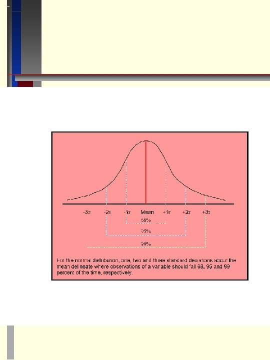
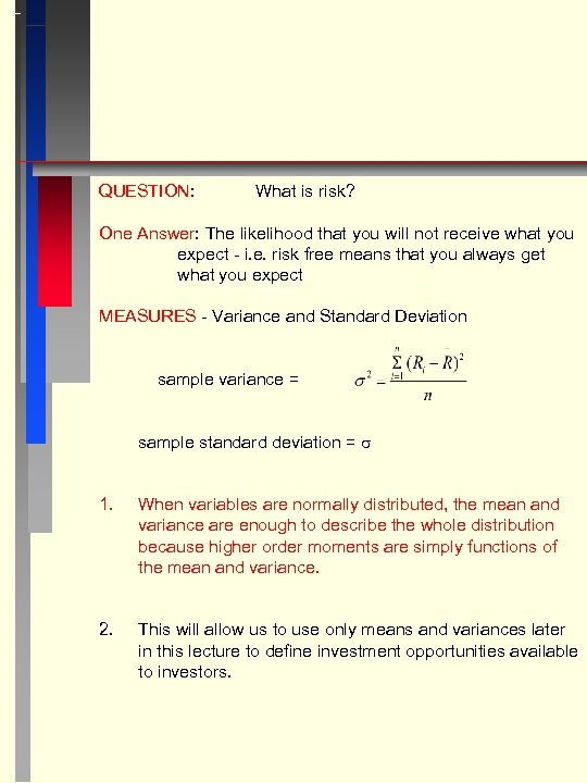QUESTION: What is risk? One Answer: The likelihood that you will not receive what you expect - i. e. risk free means that you always get what you expect MEASURES - Variance and Standard Deviation sample variance = sample standard deviation = 1. When variables are normally distributed, the mean and variance are enough to describe the whole distribution because higher order moments are simply functions of the mean and variance. 2. This will allow us to use only means and variances later in this lecture to define investment opportunities available to investors.

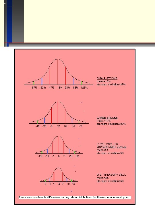
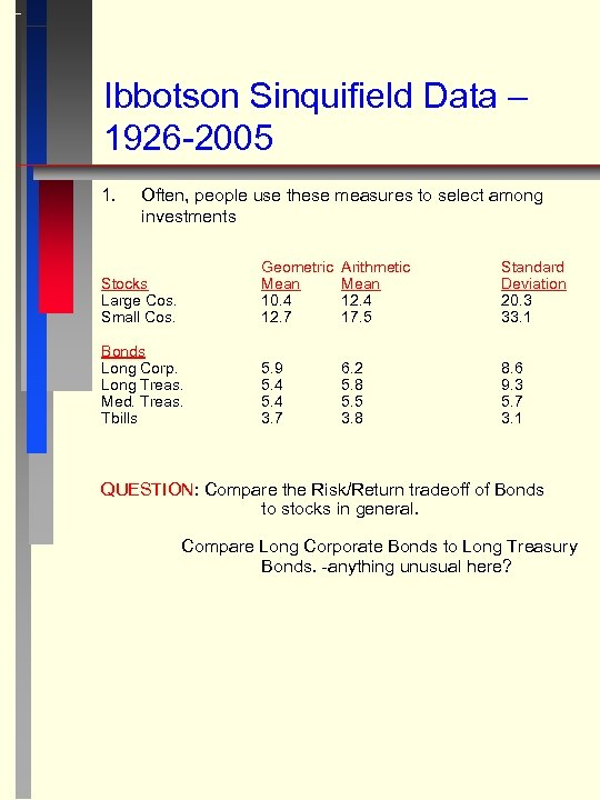Ibbotson Sinquifield Data – 1926 -2005 1. Often, people use these measures to select among investments Stocks Large Cos. Small Cos. Geometric Mean 10. 4 12. 7 Arithmetic Mean 12. 4 17. 5 Standard Deviation 20. 3 33. 1 Bonds Long Corp. Long Treas. Med. Treas. Tbills 5. 9 5. 4 3. 7 6. 2 5. 8 5. 5 3. 8 8. 6 9. 3 5. 7 3. 1 QUESTION: Compare the Risk/Return tradeoff of Bonds to stocks in general. Compare Long Corporate Bonds to Long Treasury Bonds. -anything unusual here?

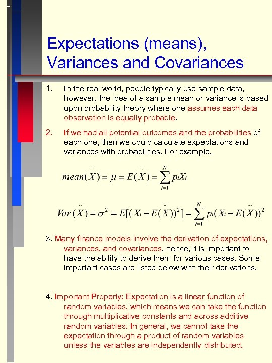Expectations (means), Variances and Covariances 1. In the real world, people typically use sample data, however, the idea of a sample mean or variance is based upon probability theory where one assumes each data observation is equally probable. 2. If we had all potential outcomes and the probabilities of each one, then we could calculate expectations and variances with probabilities. For example, 3. Many finance models involve the derivation of expectations, variances, and covariances, hence, it is important to have the ability to derive them for various cases. Some important cases are listed below with their derivations. 4. Important Property: Expectation is a linear function of random variables, which means we can take the function through multiplicative constants and across additive random variables. In general, we cannot take the expectation through a product of random variables unless the variables are independently distributed.

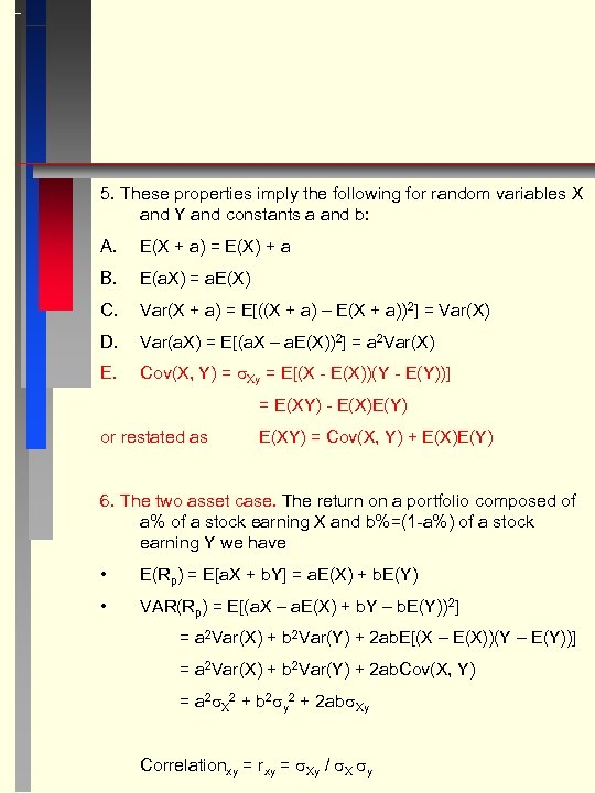5. These properties imply the following for random variables X and Y and constants a and b: A. E(X + a) = E(X) + a B. E(a. X) = a. E(X) C. Var(X + a) = E[((X + a) – E(X + a))2] = Var(X) D. Var(a. X) = E[(a. X – a. E(X))2] = a 2 Var(X) E. Cov(X, Y) = Xy = E[(X - E(X))(Y - E(Y))] = E(XY) - E(X)E(Y) or restated as E(XY) = Cov(X, Y) + E(X)E(Y) 6. The two asset case. The return on a portfolio composed of a% of a stock earning X and b%=(1 -a%) of a stock earning Y we have • E(Rp) = E[a. X + b. Y] = a. E(X) + b. E(Y) • VAR(Rp) = E[(a. X – a. E(X) + b. Y – b. E(Y))2] = a 2 Var(X) + b 2 Var(Y) + 2 ab. E[(X – E(X))(Y – E(Y))] = a 2 Var(X) + b 2 Var(Y) + 2 ab. Cov(X, Y) = a 2 X 2 + b 2 y 2 + 2 ab Xy Correlationxy = rxy = Xy / X y

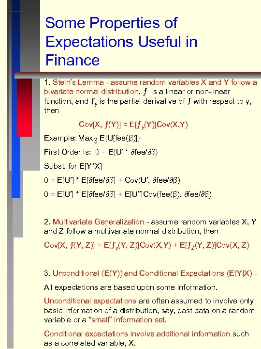Some Properties of Expectations Useful in Finance 1. Stein’s Lemma - assume random variables X and Y follow a bivariate normal distribution, ƒ is a linear or non-linear function, and ƒy is the partial derivative of ƒ with respect to y, then Cov[X, ƒ(Y)] = E[ƒy(Y)]Cov(X, Y) Example: Maxβ E{U[fee(β)]} First Order is: 0 = E{U’ * ∂fee/∂β} Subst. for E[Y*X] 0 = E[U’] * E[∂fee/∂β] + Cov(U’, ∂fee/∂β) 0 = E[U’] * E[∂fee/∂β] + E[U’’]Cov(fee(β), ∂fee/∂β) 2. Multivariate Generalization - assume random variables X, Y and Z follow a multivariate normal distribution, then Cov[X, ƒ(Y, Z)] = E[ƒy(Y, Z)]Cov(X, Y) + E[ƒZ(Y, Z)]Cov(X, Z) 3. Unconditional (E(Y)) and Conditional Expectations (E(Y|X) All expectations are based upon some information. Unconditional expectations are often assumed to involve only basic information of a distribution, say, past data on a random variable or a “small” information set. Conditional expectations involve additional information such as a correlated variable, X.

4. Law of Iterated Expectations - expectations of expectations E[E(Y|X)] = E(Y) (1) E[E(Y)|X] =E(Y) (2) 5. Restatement of L. I. E. - when you take expectations of expectations, the expectations conditional on the least information of the two (unconditional expectations) prevails. This is useful in cases where you must forecast the behavior of others with a different information set or get some average of a set of conditional expectations. 6. Concrete Example - Suppose you want to predict whether a risk-neutral investor faced with the choice between buying stock with return R or bonds with return B will buy stock today. Assume that everyone knows that 60% of the time R > B. For the two cases, (1) and (2), either the investor or you get a signal X that says R < B for sure today : Equation (1) says, if the investor gets the signal, then you should still predict the investor will buy stock (the unconditional expectation). Since you don’t have the information, you go with the lesser informed prediction. Of course, you will be wrong in this case but there was no way for you to know this beforehand. Equation (2) says, if the you get the signal then you predict the investor will buy stock (again, the unconditional expectation). Here, your prediction will be correct even though you know that had the investor known what you knew, he would not buy stock.

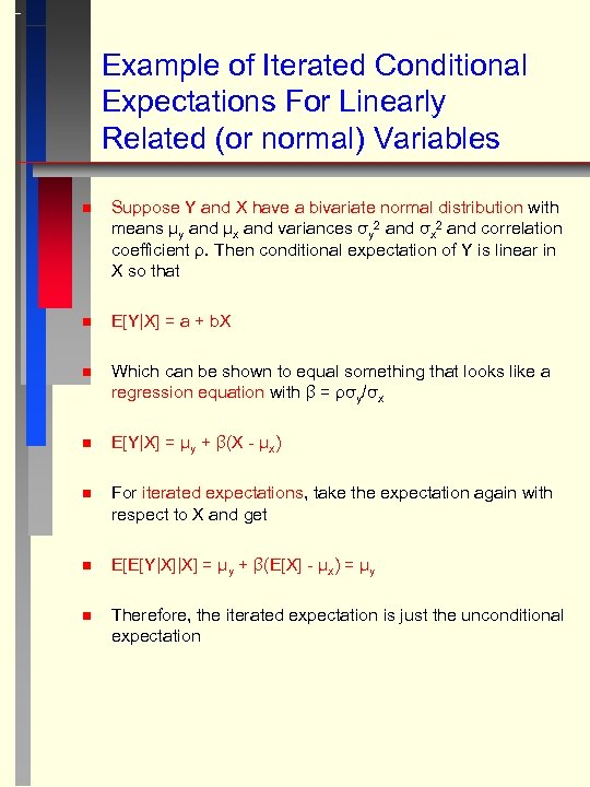Example of Iterated Conditional Expectations For Linearly Related (or normal) Variables n Suppose Y and X have a bivariate normal distribution with means µy and µx and variances σy 2 and σx 2 and correlation coefficient ρ. Then conditional expectation of Y is linear in X so that n E[Y|X] = a + b. X n Which can be shown to equal something that looks like a regression equation with β = ρσy/σx n E[Y|X] = µy + β(X - µx) n For iterated expectations, take the expectation again with respect to X and get n E[E[Y|X]|X] = µy + β(E[X] - µx) = µy n Therefore, the iterated expectation is just the unconditional expectation

Intermediate steps for previous slide n E[Y|X] = a + b. X n Integrating (taking expectations) over X gives n E[Y] = a + b. E[X] µy = a + b µx n n n or Now consider the expectation of the product E[Y|X]X = a. X + b. X 2 Integrating over X gives E[YX] = a. E[X] + b. E[X 2] n Using the definition of Cov[Y, X] = ρσyσx = E[YX] - µy µx and E[X 2] = σx 2 + µx 2 (see next few slides) then n ρσyσx + µy µx = a µx + b(σx 2 + µx 2 ) n Use this and µy = a + b µx to solve for a and b as a = µy – µxρσy/σx and b = ρσy/σx n n E[Y|X] = µy + ρσy/σx (X - µx)

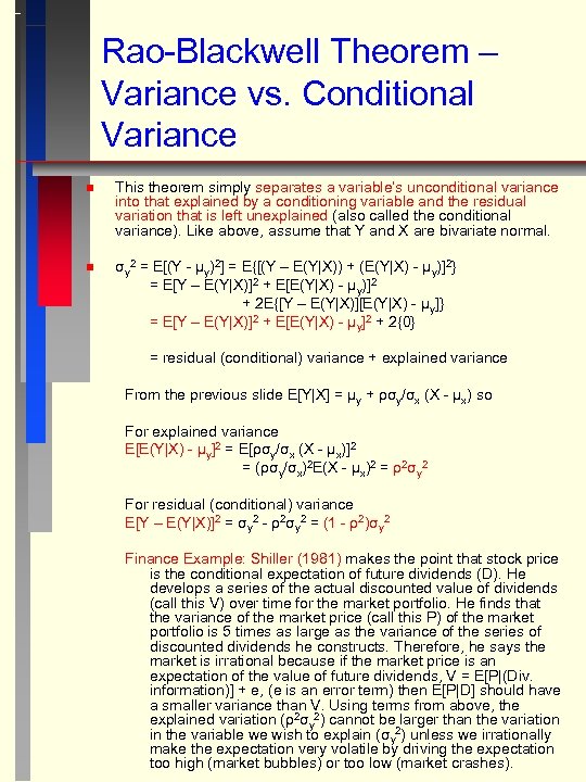Rao-Blackwell Theorem – Variance vs. Conditional Variance n This theorem simply separates a variable’s unconditional variance into that explained by a conditioning variable and the residual variation that is left unexplained (also called the conditional variance). Like above, assume that Y and X are bivariate normal. n σy 2 = E[(Y - µy)2] = E{[(Y – E(Y|X)) + (E(Y|X) - µy)]2} = E[Y – E(Y|X)]2 + E[E(Y|X) - µy)]2 + 2 E{[Y – E(Y|X)][E(Y|X) - µy]} = E[Y – E(Y|X)]2 + E[E(Y|X) - µy]2 + 2{0} = residual (conditional) variance + explained variance From the previous slide E[Y|X] = µy + ρσy/σx (X - µx) so For explained variance E[E(Y|X) - µy]2 = E[ρσy/σx (X - µx)]2 = (ρσy/σx)2 E(X - µx)2 = ρ2σy 2 For residual (conditional) variance E[Y – E(Y|X)]2 = σy 2 - ρ2σy 2 = (1 - ρ2)σy 2 Finance Example: Shiller (1981) makes the point that stock price is the conditional expectation of future dividends (D). He develops a series of the actual discounted value of dividends (call this V) over time for the market portfolio. He finds that the variance of the market price (call this P) of the market portfolio is 5 times as large as the variance of the series of discounted dividends he constructs. Therefore, he says the market is irrational because if the market price is an expectation of the value of future dividends, V = E[P|(Div. information)] + e, (e is an error term) then E[P|D] should have a smaller variance than V. Using terms from above, the explained variation (ρ2σy 2) cannot be larger than the variation in the variable we wish to explain (σy 2) unless we irrationally make the expectation very volatile by driving the expectation too high (market bubbles) or too low (market crashes).

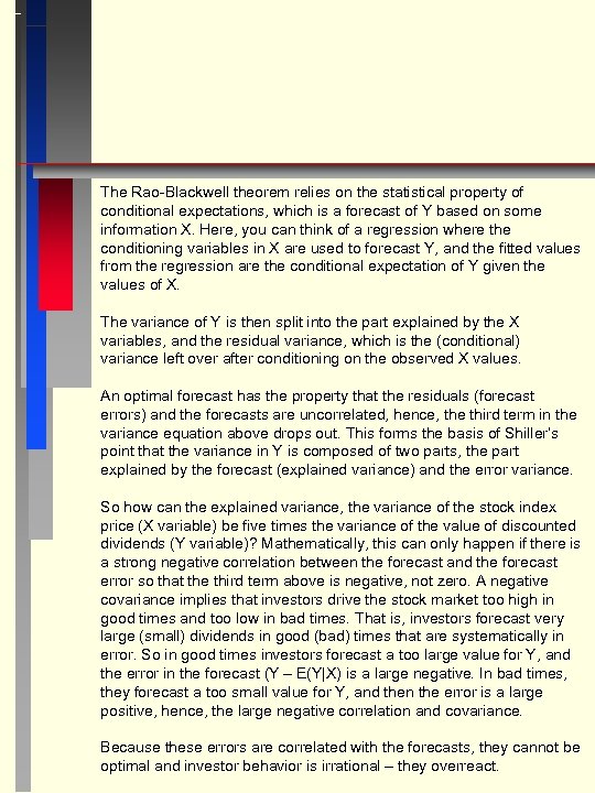The Rao-Blackwell theorem relies on the statistical property of conditional expectations, which is a forecast of Y based on some information X. Here, you can think of a regression where the conditioning variables in X are used to forecast Y, and the fitted values from the regression are the conditional expectation of Y given the values of X. The variance of Y is then split into the part explained by the X variables, and the residual variance, which is the (conditional) variance left over after conditioning on the observed X values. An optimal forecast has the property that the residuals (forecast errors) and the forecasts are uncorrelated, hence, the third term in the variance equation above drops out. This forms the basis of Shiller’s point that the variance in Y is composed of two parts, the part explained by the forecast (explained variance) and the error variance. So how can the explained variance, the variance of the stock index price (X variable) be five times the variance of the value of discounted dividends (Y variable)? Mathematically, this can only happen if there is a strong negative correlation between the forecast and the forecast error so that the third term above is negative, not zero. A negative covariance implies that investors drive the stock market too high in good times and too low in bad times. That is, investors forecast very large (small) dividends in good (bad) times that are systematically in error. So in good times investors forecast a too large value for Y, and the error in the forecast (Y – E(Y|X) is a large negative. In bad times, they forecast a too small value for Y, and then the error is a large positive, hence, the large negative correlation and covariance. Because these errors are correlated with the forecasts, they cannot be optimal and investor behavior is irrational – they overreact.

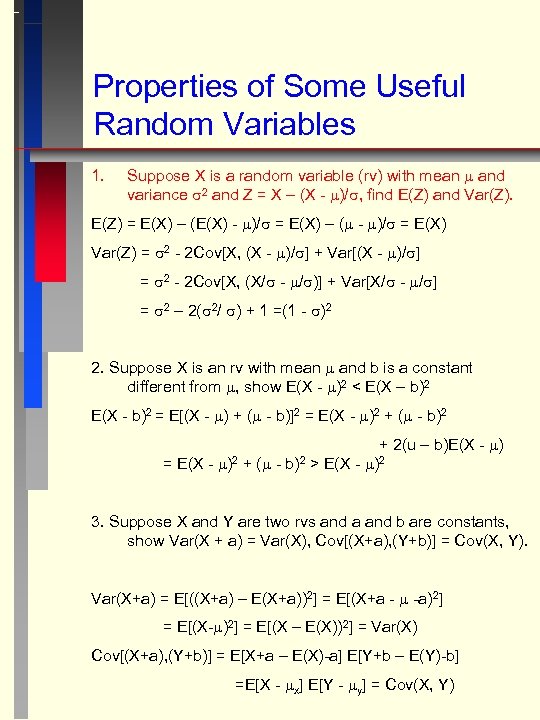Properties of Some Useful Random Variables 1. Suppose X is a random variable (rv) with mean and variance 2 and Z = X – (X - )/ , find E(Z) and Var(Z). E(Z) = E(X) – (E(X) - )/ = E(X) – ( - )/ = E(X) Var(Z) = 2 - 2 Cov[X, (X - )/ ] + Var[(X - )/ ] = 2 - 2 Cov[X, (X/ - / )] + Var[X/ - / ] = 2 – 2( 2/ ) + 1 =(1 - )2 2. Suppose X is an rv with mean and b is a constant different from , show E(X - )2 < E(X – b)2 E(X - b)2 = E[(X - ) + ( - b)]2 = E(X - )2 + ( - b)2 + 2(u – b)E(X - ) = E(X - )2 + ( - b)2 > E(X - )2 3. Suppose X and Y are two rvs and a and b are constants, show Var(X + a) = Var(X), Cov[(X+a), (Y+b)] = Cov(X, Y). Var(X+a) = E[((X+a) – E(X+a))2] = E[(X+a - -a)2] = E[(X- )2] = E[(X – E(X))2] = Var(X) Cov[(X+a), (Y+b)] = E[X+a – E(X)-a] E[Y+b – E(Y)-b] =E[X - x] E[Y - y] = Cov(X, Y)

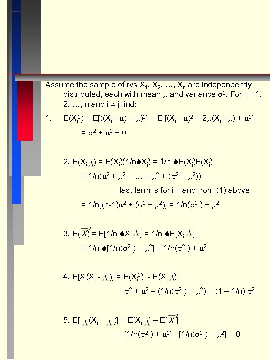Assume the sample of rvs X 1, X 2, …, Xn are independently distributed, each with mean and variance 2. For i = 1, 2, …, n and i j find: 1. E(Xi 2) = E[((Xi - ) + )2] = E [(Xi - )2 + 2 (Xi - ) + 2] = 2 + 0 2. E(Xi ) = E(Xi)(1/n Xj) = 1/n E(Xj) = 1/n( 2 + … + 2 + ( 2 + 2)) last term is for i=j and from (1) above = 1/n[(n-1) 2 + ( 2 + 2)] = 1/n( 2 ) + 2 3. E( ) = E[1/n Xi ] = 1/n E[Xi ] = 1/n [1/n( 2 ) + 2] = 1/n( 2 ) + 2 4. E[Xi(Xi - )] = E(Xi 2) - E(Xi ) = 2 + 2 – (1/n( 2 ) + 2) = (1 – 1/n) 2 5. E[ (Xi - )] = E[Xi ] – E[ ] = [1/n( 2 ) + 2] - [1/n( 2 ) + 2] = 0

)] = E(Xi. Xj) - E(Xi ) = 2 - [1/n( 2 ) + 2] 6. E[Xi(Xj - = - 1/n( 2 ) 7. Cov[Xi, ] = Cov[ Xi, 1/n Xj ] = (1/n)Cov[Xi, Xi] + (1/n) Cov[Xi, j i. Xj] = 1/n( 2) 8. Var[Xi - ] = Var[Xi] - 2 Cov[Xi, = 2 – 2(1/n)( 2 ) + E[( ] + Var[ ] - )2] = 2 – 2(1/n)( 2 ) + E[(1/n Xj - )2] = 2 – 2(1/n)( 2 ) + 1/n 2 E(Xj - )2] = 2 – 2(1/n)( 2 ) + 1/n 2(n 2 )] = 2 – 2(1/n)( 2 ) + 1/n( 2 ) = 2 (1 – 1/n) 9. Cov [(Xi - ), ] = Cov[Xi, ] – Cov[ , ] – Var[ ] ] = 1/n( 2) - 1/n( 2 ) = 0 10. Cov [(Xi - ), (Xj - )] = Cov[Xi, Xj] - Cov[Xi, ] + Var[ = 0 - 1/n( 2) + 1/n( 2) = -1/n( 2) ] ]

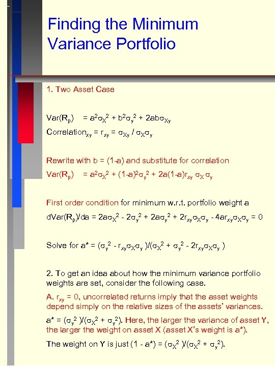Finding the Minimum Variance Portfolio 1. Two Asset Case Var(Rp) = a 2 X 2 + b 2 y 2 + 2 ab Xy Correlationxy = rxy = Xy / X y Rewrite with b = (1 -a) and substitute for correlation Var(Rp) = a 2 X 2 + (1 -a)2 y 2 + 2 a(1 -a)rxy X y First order condition for minimum w. r. t. portfolio weight a d. Var(Rp)/da = 2 a X 2 - 2 y 2 + 2 a y 2 + 2 rxy X y - 4 arxy X y = 0 Solve for a* = ( y 2 - rxy X y )/( X 2 + y 2 - 2 rxy X y ) 2. To get an idea about how the minimum variance portfolio weights are set, consider the following case. A. rxy = 0, uncorrelated returns imply that the asset weights depend simply on the relative sizes of the assets’ variances. a* = ( y 2 )/( X 2 + y 2). Here, the larger the variance of asset Y, the larger the weight on asset X (asset X’s weight is a*). The weight on Y is just (1 - a*) = ( X 2 )/( X 2 + y 2).

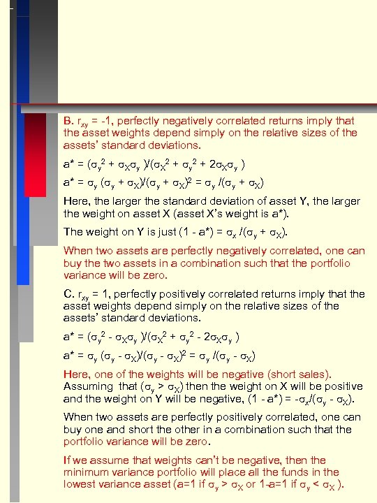B. rxy = -1, perfectly negatively correlated returns imply that the asset weights depend simply on the relative sizes of the assets’ standard deviations. a* = ( y 2 + X y )/( X 2 + y 2 + 2 X y ) a* = y ( y + X)/( y + X)2 = y /( y + X) Here, the larger the standard deviation of asset Y, the larger the weight on asset X (asset X’s weight is a*). The weight on Y is just (1 - a*) = x /( y + X). When two assets are perfectly negatively correlated, one can buy the two assets in a combination such that the portfolio variance will be zero. C. rxy = 1, perfectly positively correlated returns imply that the asset weights depend simply on the relative sizes of the assets’ standard deviations. a* = ( y 2 - X y )/( X 2 + y 2 - 2 X y ) a* = y ( y - X)/( y - X)2 = y /( y - X) Here, one of the weights will be negative (short sales). Assuming that ( y > X) then the weight on X will be positive and the weight on Y will be negative, (1 - a*) = - x/( y - X). When two assets are perfectly positively correlated, one can buy one and short the other in a combination such that the portfolio variance will be zero. If we assume that weights can’t be negative, then the minimum variance portfolio will place all the funds in the lowest variance asset (a=1 if y > X or 1 -a=1 if y < X ).

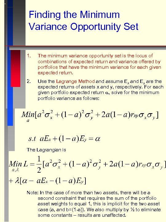Finding the Minimum Variance Opportunity Set 1. The minimum variance opportunity set is the locus of combinations of expected return and variance offered by portfolios that have the minimum variance for each given expected return. 2. Use the Lagrange Method and assume Ex and Ey are the expected returns of assets x and y, respectively. For each given portfolio expected return , solve for the minimum portfolio variance as follows: The Lagrangian is Note: In the case of more than two assets, there will be a second constraint that requires the sum of the portfolio asset weights to equal 1, this is implicit for the two asset case (a, and b=(1 -a)). We also multiply by ½ to eliminate some constants – results are unaffected.

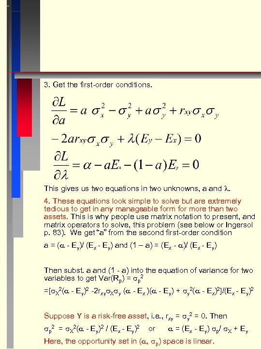3. Get the first-order conditions. This gives us two equations in two unknowns, a and . 4. These equations look simple to solve but are extremely tedious to get in any manageable form for more than two assets. This is why people use matrix notation to present, and matrix operators to solve, this problem (see below or Ingersol p. 83). We get “a” from the second first-order condition a = ( - Ey)/ (Ex - Ey) and (1 – a) = (Ex - )/ (Ex - Ey) Then subst. a and (1 - a) into the equation of variance for two variables to get Var(Rp) = p 2 =[ X 2( - Ey)2 -2 rxy X y ( - Ex )( - Ey) + y 2( - Ex)2]/(Ex - Ey)2 Suppose Y is a risk-free asset, i. e. , rxy = y 2 = 0. Then p 2 = X 2( - Ey)2 / (Ex - Ey)2 or = (Ex - Ey) p/ X + Ey Here, the opportunity set in ( , p) space is linear.

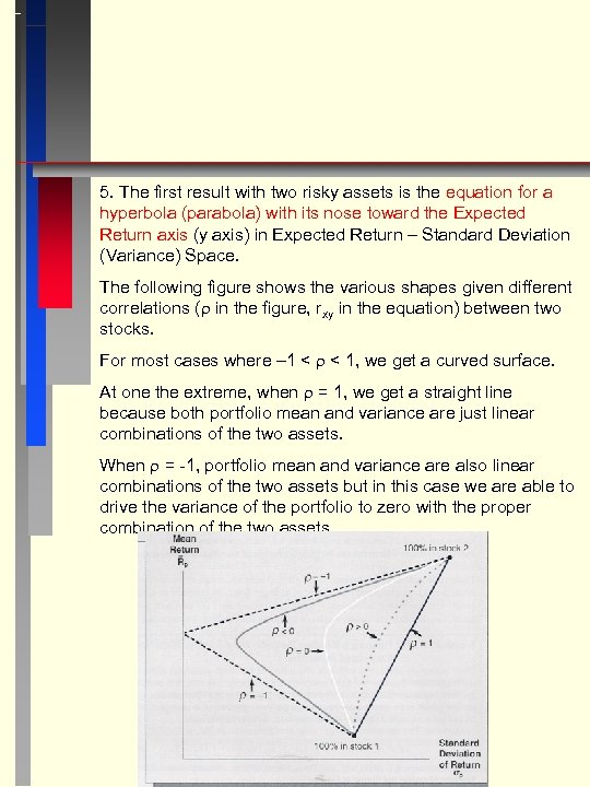5. The first result with two risky assets is the equation for a hyperbola (parabola) with its nose toward the Expected Return axis (y axis) in Expected Return – Standard Deviation (Variance) Space. The following figure shows the various shapes given different correlations ( in the figure, rxy in the equation) between two stocks. For most cases where – 1 < < 1, we get a curved surface. At one the extreme, when = 1, we get a straight line because both portfolio mean and variance are just linear combinations of the two assets. When = -1, portfolio mean and variance are also linear combinations of the two assets but in this case we are able to drive the variance of the portfolio to zero with the proper combination of the two assets.

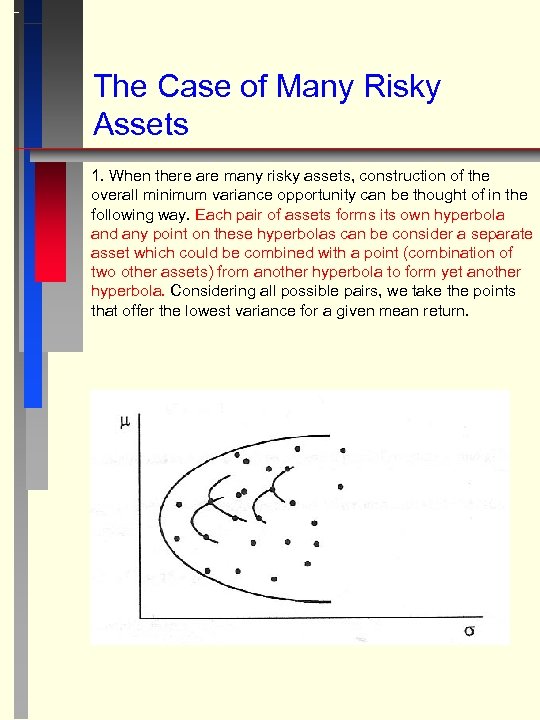The Case of Many Risky Assets 1. When there are many risky assets, construction of the overall minimum variance opportunity can be thought of in the following way. Each pair of assets forms its own hyperbola and any point on these hyperbolas can be consider a separate asset which could be combined with a point (combination of two other assets) from another hyperbola to form yet another hyperbola. Considering all possible pairs, we take the points that offer the lowest variance for a given mean return.

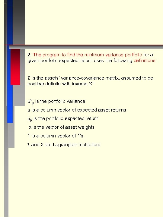2. The program to find the minimum variance portfolio for a given portfolio expected return uses the following definitions is the assets’ variance-covariance matrix, assumed to be positive definite with inverse -1 2 p is the portfolio variance is a column vector of expected asset returns p is the portfolio expected return x is the vector of asset weights 1 is a column vector of 1’s and are Lagrangian multipliers

Minx [½ x’ x] = 2 p s. t. ‘ x = p and 1’x = 1 The Lagrangian is Min L = [½ x’ x] + [ p - ‘ x ] + [1 - 1’x] The first-order condition w. r. t. x is x’ - ‘ - 1’ = 0 Solving for the optimal portfolio asset weights x’ = ‘ -1 + 1’ -1 Using f. o. c. again, post-multiply by x and use the constraints 2 p = p + Now we need to find and to get the portfolio frontier.

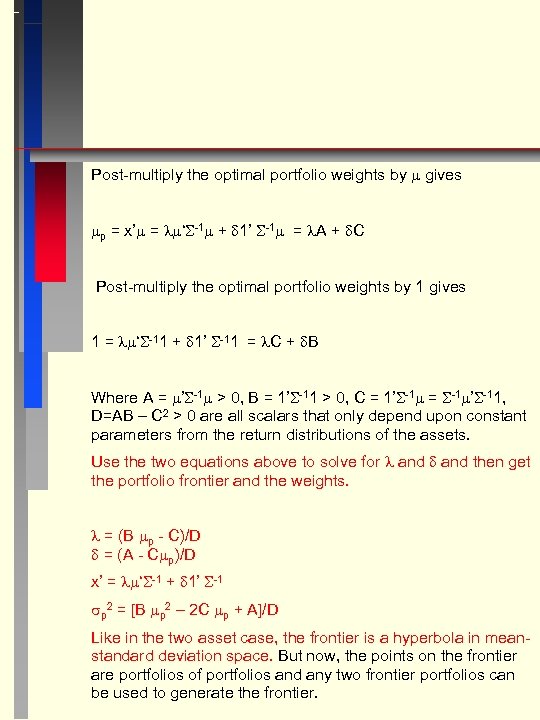Post-multiply the optimal portfolio weights by gives p = x’ = ‘ -1 + 1’ -1 = A + C Post-multiply the optimal portfolio weights by 1 gives 1 = ‘ -11 + 1’ -11 = C + B Where A = ’ -1 > 0, B = 1’ -11 > 0, C = 1’ -1 = -1 ’ -11, D=AB – C 2 > 0 are all scalars that only depend upon constant parameters from the return distributions of the assets. Use the two equations above to solve for and then get the portfolio frontier and the weights. = (B p - C)/D = (A - C p)/D x’ = ‘ -1 + 1’ -1 p 2 = [B p 2 – 2 C p + A]/D Like in the two asset case, the frontier is a hyperbola in meanstandard deviation space. But now, the points on the frontier are portfolios of portfolios and any two frontier portfolios can be used to generate the frontier.

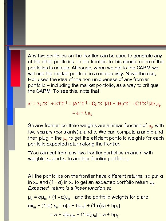Any two portfolios on the frontier can be used to generate any of the other portfolios on the frontier. In this sense, none of the portfolios is unique. Although, when we get to the CAPM we will use the market portfolio in a unique way. Nevertheless, Roll used the idea of the non-uniqueness of any frontier portfolio – including the market portfolio, as a way to critique the CAPM. To see this, note that x’ = ‘ -1 + 1’ -1 = [A 1’ -1 - C ‘ -1]/D + [B ‘ -1 - C 1’ -1]/D p = a + b p So any frontier portfolio weights are a linear function of p with two scalars (constants) a and b. We can compute a and b and then plug in the p to get the efficient portfolio weights for each portfolio expected return along the frontier. *You can get from any two frontier portfolios m and n with weights xm and xn to another frontier portfolio p. All the portfolios on the frontier have different returns, so put α in xm and (1 - α) in xn to get an expected portfolio return μp. Expected return is a linear function so μp = αμm + (1 - α)μn and the portfolio weights for p are αxm + (1 -α) xn = α[a + bμm] + (1 -α)[a + bμn] = a + b[αμm + (1 -α)μn] = a + bμp

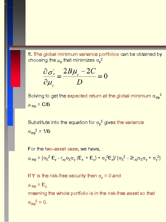8. The global minimum variance portfolios can be obtained by choosing the p that minimizes p 2 Solving to get the expected return at the global minimum mp 2 mp = C/B Substitute into the equation for p 2 gives the variance mp 2 = 1/B For the two-asset case, we have, mp = [ X 2 Ey - rxy X y (Ex + Ey) + y 2 Ex]/ [ X 2 - 2 rxy X y + y 2] If Y is the risk-free security then y = 0 and mp = Ey meaning the whole portfolio is in the risk-free asset so that mp 2 = 0.

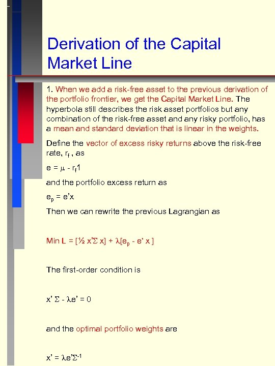Derivation of the Capital Market Line 1. When we add a risk-free asset to the previous derivation of the portfolio frontier, we get the Capital Market Line. The hyperbola still describes the risk asset portfolios but any combination of the risk-free asset and any risky portfolio, has a mean and standard deviation that is linear in the weights. Define the vector of excess risky returns above the risk-free rate, rf , as e = - rf 1 and the portfolio excess return as ep = e’x Then we can rewrite the previous Lagrangian as Min L = [½ x’ x] + [ep - e‘ x ] The first-order condition is x’ - e’ = 0 and the optimal portfolio weights are x’ = e’ -1

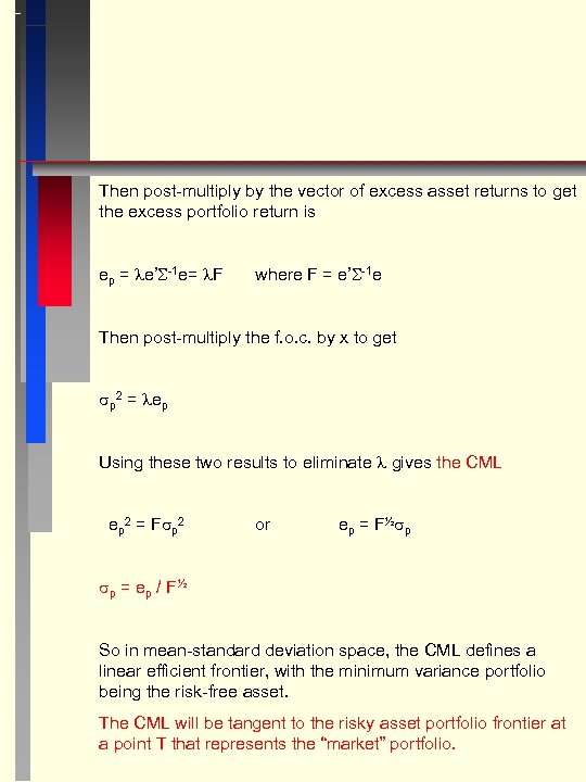Then post-multiply by the vector of excess asset returns to get the excess portfolio return is ep = e’ -1 e= F where F = e’ -1 e Then post-multiply the f. o. c. by x to get p 2 = ep Using these two results to eliminate gives the CML ep 2 = F p 2 or ep = F½ p p = e p / F ½ So in mean-standard deviation space, the CML defines a linear efficient frontier, with the minimum variance portfolio being the risk-free asset. The CML will be tangent to the risky asset portfolio frontier at a point T that represents the “market” portfolio.

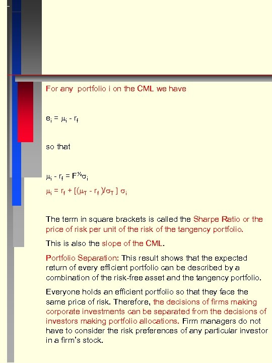For any portfolio i on the CML we have e i = i - rf so that i - rf = F½ i i = rf + [( T - rf )/ T ] i The term in square brackets is called the Sharpe Ratio or the price of risk per unit of the risk of the tangency portfolio. This is also the slope of the CML. Portfolio Separation: This result shows that the expected return of every efficient portfolio can be described by a combination of the risk-free asset and the tangency portfolio. Everyone holds an efficient portfolio so that they face the same price of risk. Therefore, the decisions of firms making corporate investments can be separated from the decisions of investors making portfolio allocations. Firm managers do not have to consider the risk preferences of any particular investor in a firm’s stock.

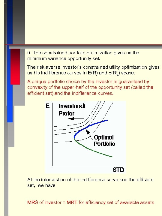9. The constrained portfolio optimization gives us the minimum variance opportunity set. The risk averse investor’s constrained utility optimization gives us his indifference curves in E(R) and (Rp) space. A unique portfolio choice by the investor is guaranteed by convexity of the upper-half of the opportunity set (called the efficient set) and the indifference curves. At the intersection of the indifference curve and the efficient set, we have MRS of investor = MRT for efficiency set of available assets

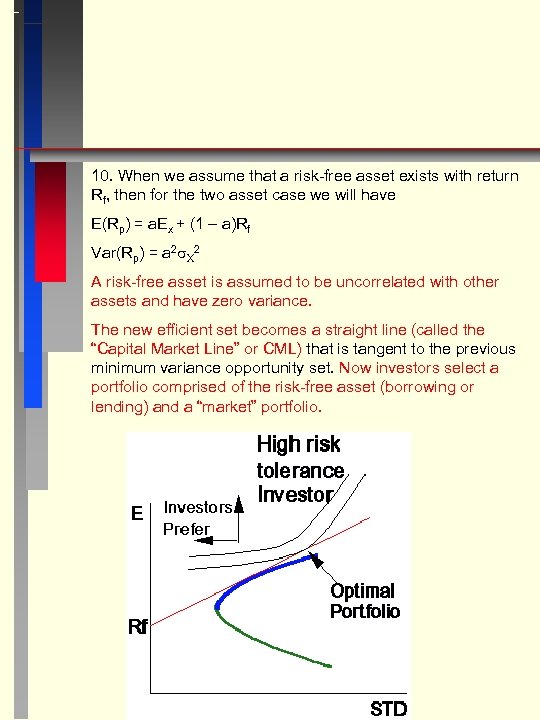10. When we assume that a risk-free asset exists with return Rf, then for the two asset case we will have E(Rp) = a. Ex + (1 – a)Rf Var(Rp) = a 2 X 2 A risk-free asset is assumed to be uncorrelated with other assets and have zero variance. The new efficient set becomes a straight line (called the “Capital Market Line” or CML) that is tangent to the previous minimum variance opportunity set. Now investors select a portfolio comprised of the risk-free asset (borrowing or lending) and a “market” portfolio.

11. Note that points along the CML are linear combinations of the risk free rate and a portfolio defined by the tangency between the CML and the investment opportunity set. If all investors have the same beliefs about the return distributions of the assets, then this tangency portfolio is the “market” portfolio and the CML can be defined from the fact that the slopes of the CML and opportunity set must be equal at the tangency so Slope of CML = Slope of Opportunity set [E(Rp) - Rf ] / [E(RM) – Rf] = p / M Rearranging gives E(Rp) = Rf + [E(RM) – Rf] p / M The second term on the RHS is the product of the units of risk ( p ) and the price of risk [E(RM) – Rf]/ M. Two-Fund Separation: As a result, all portfolios are defined by the risk-free security and the market portfolio. This implies that for all investors MRS of any investor = MRT from the CML = [E(RM) – Rf]/ M All investors agree on the price of risk. This implies that investment decisions can be “separated” from the particular risk preferences of a firm’s investors. Managers of firms can use the market equilibrium price of risk to evaluate potential investments rather than define the particular risk preferences of their investors.

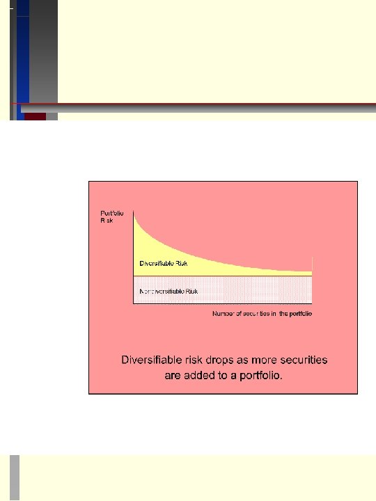
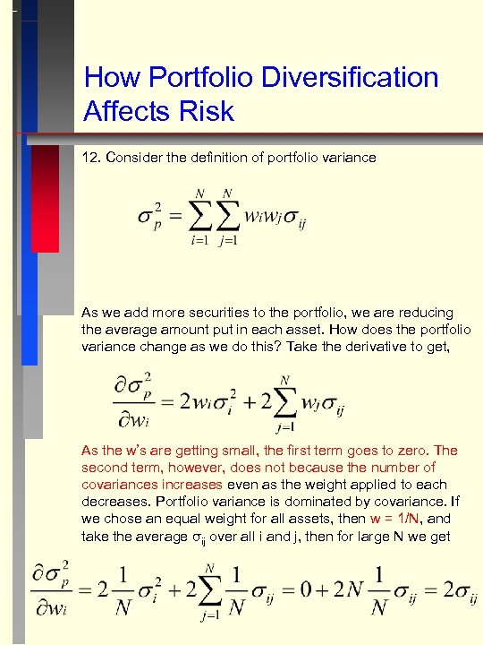How Portfolio Diversification Affects Risk 12. Consider the definition of portfolio variance As we add more securities to the portfolio, we are reducing the average amount put in each asset. How does the portfolio variance change as we do this? Take the derivative to get, As the w’s are getting small, the first term goes to zero. The second term, however, does not because the number of covariances increases even as the weight applied to each decreases. Portfolio variance is dominated by covariance. If we chose an equal weight for all assets, then w = 1/N, and take the average σij over all i and j, then for large N we get

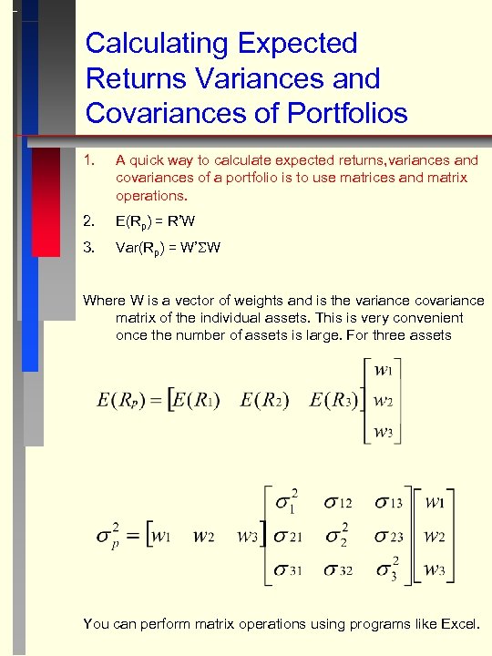Calculating Expected Returns Variances and Covariances of Portfolios 1. A quick way to calculate expected returns, variances and covariances of a portfolio is to use matrices and matrix operations. 2. E(Rp) = R’W 3. Var(Rp) = W’ W Where W is a vector of weights and is the variance covariance matrix of the individual assets. This is very convenient once the number of assets is large. For three assets You can perform matrix operations using programs like Excel.

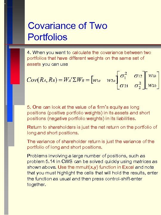Covariance of Two Portfolios 4. When you want to calculate the covariance between two portfolios that have different weights on the same set of assets you can use 5. One can look at the value of a firm’s equity as long positions (positive portfolio weights) in its assets and short positions (negative portfolio weights) in its liabilities. Return to shareholders is just the net return on the portfolio of long and short positions. The variance of shareholder return is just the variance of the portfolio of long and short positions. Problems involving a large number of positions, such as problem 5. 14 in CWS can be solved quickly using matrices as shown above. Use the mmult(x, y) function in Excel and note that you must highlight the cells that will hold the results, enter the function as usual and then press control-shift-enter together.