Requirements-based Test Generation Professor W Eric Wong Department

Requirements-based Test Generation Professor W. Eric Wong Department of Computer Science University of Texas at Dallas http: //www. utdallas. edu/~ewong/sysm 6367. html

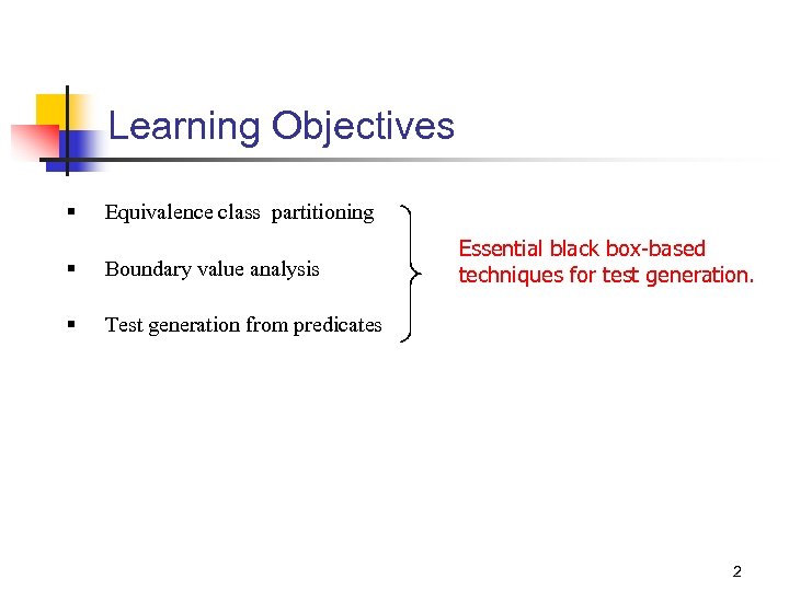
Learning Objectives § Equivalence class partitioning § Boundary value analysis § Essential black box-based techniques for test generation. Test generation from predicates 2

Test generation techniques described in this unit belong to the black-box testing category. These techniques are useful during functional testing where the objective is to test whether or not an application, unit, system, or subsystem, correctly implements the functionality as per the given requirements 3

The Test Selection Problem 4

Requirements and Test Generation Requirements serve as the starting point for the generation of tests. During the initial phases of development, requirements may exist only in the minds of one or more people. These requirements, more aptly ideas, are then specified rigorously using modeling elements such as use cases, sequence diagrams, and statecharts in UML. Rigorously specified requirements are often transformed into formal requirements using requirements specification languages such as Z. 5

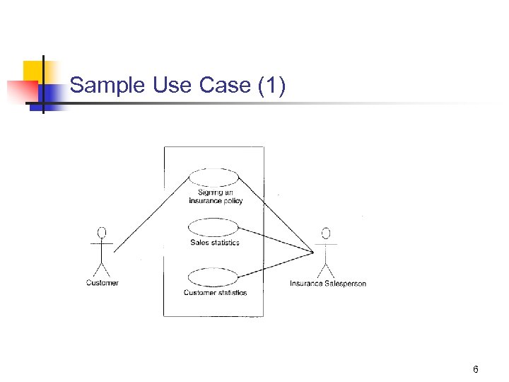
Sample Use Case (1) 6

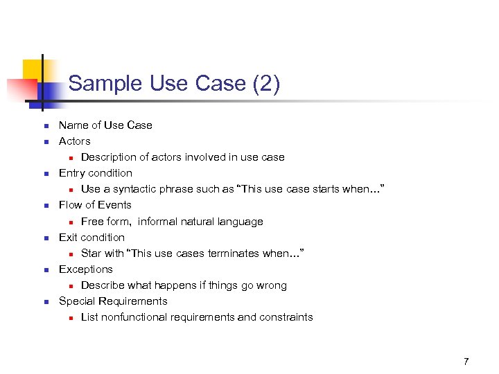
Sample Use Case (2) n n n n Name of Use Case Actors n Description of actors involved in use case Entry condition n Use a syntactic phrase such as “This use case starts when…” Flow of Events n Free form, informal natural language Exit condition n Star with “This use cases terminates when…” Exceptions n Describe what happens if things go wrong Special Requirements n List nonfunctional requirements and constraints 7

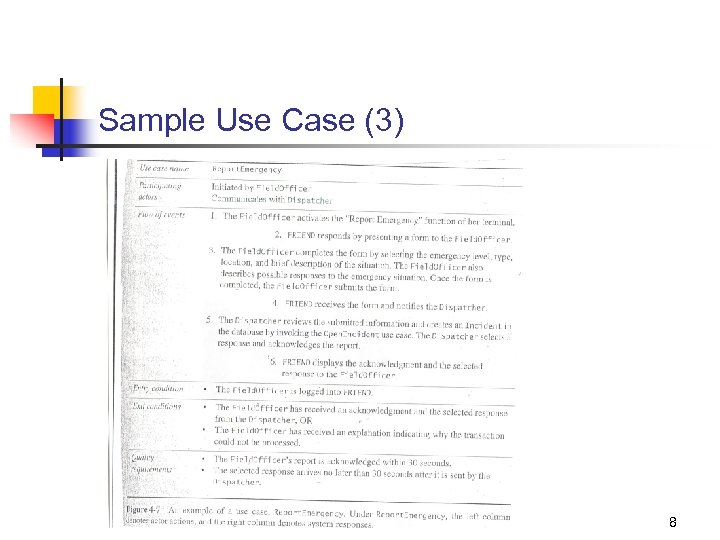
Sample Use Case (3) 8

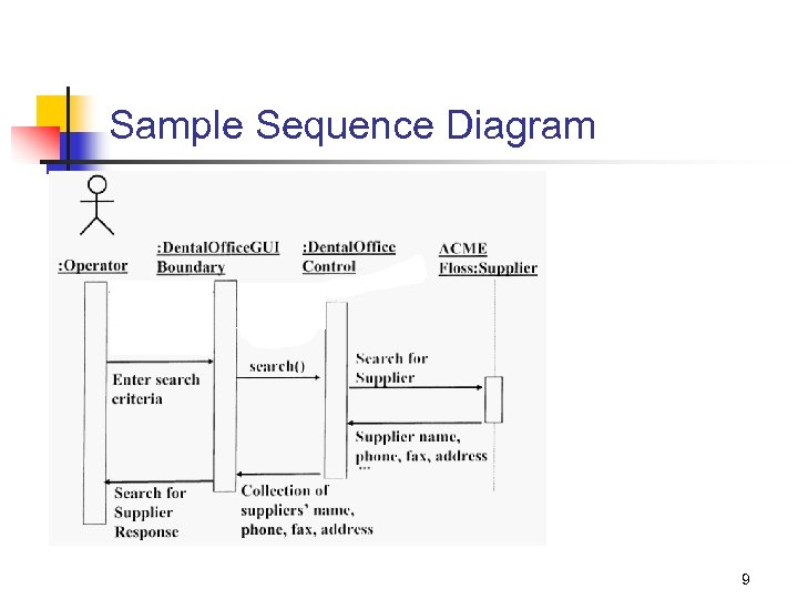
Sample Sequence Diagram 9

Test Selection Problem Let D denote the input domain of a program P. Ideally, the test selection problem is to select a subset T of tests such that execution of P against each element of T will reveal all errors in P. In general there does not exist any algorithm to construct such a test set. However, there are heuristics and model based methods that can be used to generate tests that will reveal certain type of faults. 10

Test Selection Problem (contd. ) The challenge is to construct a test set T D that will reveal as many errors in P as possible. The problem of test selection is difficult due primarily to the size and complexity of the input domain of P. 11

Exhaustive Testing The large size of the input domain prevents a tester from exhaustively testing the program under test against all possible inputs. By “exhaustive” testing we mean testing the given program against every element in its input domain. The complexity makes it harder to select individual tests. The following two examples illustrate what is responsible for large and complex input domains. 12

Large Input Domain Consider program P that is required to sort a sequence of integers into ascending order. Assuming that P will be executed on a machine in which integers range from -32768 to 32767, the input domain of P consists of all possible sequences of integers in the range [-32768, 32767]. If there is no limit on the size of the sequence that can be input, then the input domain of P is infinitely large and P can never be tested exhaustively. If the size of the input sequence is limited to, say Nmax>1, then the size of the input domain depends on the value of N. Calculate the size of the input domain 13

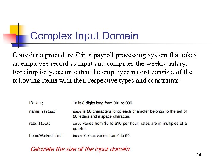
Complex Input Domain Consider a procedure P in a payroll processing system that takes an employee record as input and computes the weekly salary. For simplicity, assume that the employee record consists of the following items with their respective types and constraints: Calculate the size of the input domain 14

Equivalence Class Partitioning 15

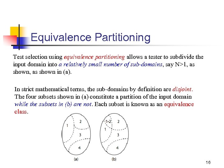
Equivalence Partitioning Test selection using equivalence partitioning allows a tester to subdivide the input domain into a relatively small number of sub-domains, say N>1, as shown in (a). In strict mathematical terms, the sub-domains by definition are disjoint. The four subsets shown in (a) constitute a partition of the input domain while the subsets in (b) are not. Each subset is known as an equivalence class. 16

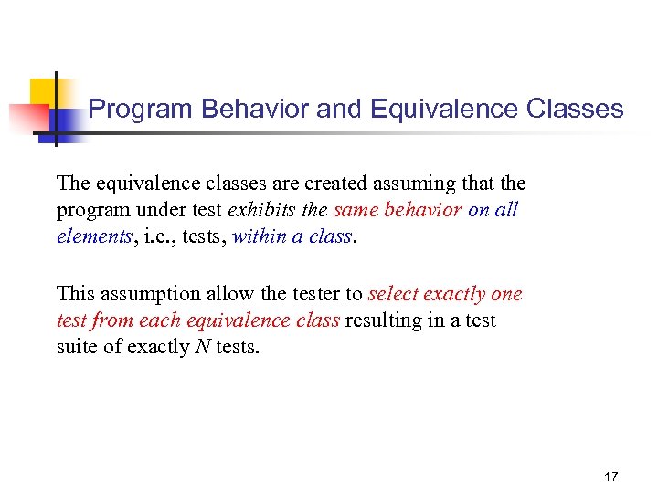
Program Behavior and Equivalence Classes The equivalence classes are created assuming that the program under test exhibits the same behavior on all elements, i. e. , tests, within a class. This assumption allow the tester to select exactly one test from each equivalence class resulting in a test suite of exactly N tests. 17

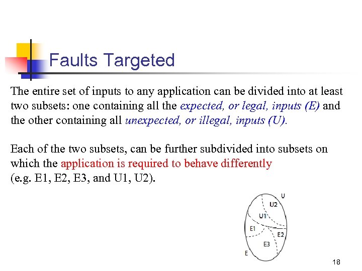
Faults Targeted The entire set of inputs to any application can be divided into at least two subsets: one containing all the expected, or legal, inputs (E) and the other containing all unexpected, or illegal, inputs (U). Each of the two subsets, can be further subdivided into subsets on which the application is required to behave differently (e. g. E 1, E 2, E 3, and U 1, U 2). 18

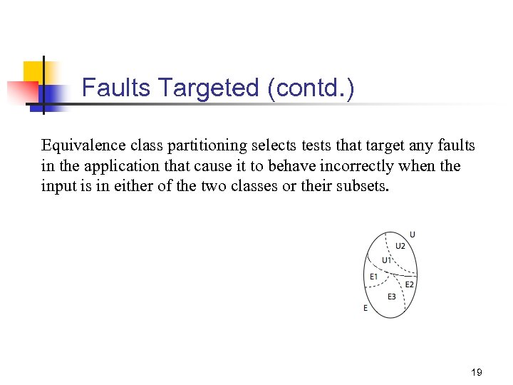
Faults Targeted (contd. ) Equivalence class partitioning selects tests that target any faults in the application that cause it to behave incorrectly when the input is in either of the two classes or their subsets. 19

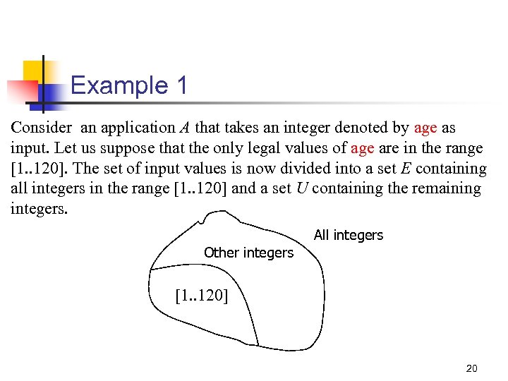
Example 1 Consider an application A that takes an integer denoted by age as input. Let us suppose that the only legal values of age are in the range [1. . 120]. The set of input values is now divided into a set E containing all integers in the range [1. . 120] and a set U containing the remaining integers. All integers Other integers [1. . 120] 20

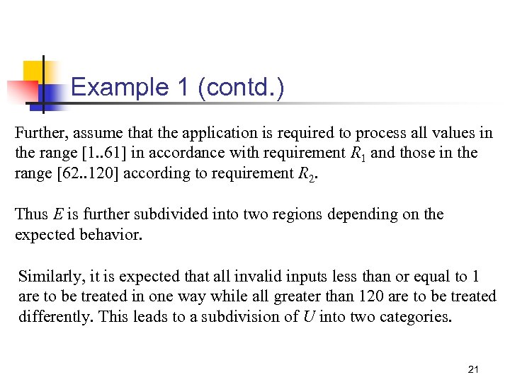
Example 1 (contd. ) Further, assume that the application is required to process all values in the range [1. . 61] in accordance with requirement R 1 and those in the range [62. . 120] according to requirement R 2. Thus E is further subdivided into two regions depending on the expected behavior. Similarly, it is expected that all invalid inputs less than or equal to 1 are to be treated in one way while all greater than 120 are to be treated differently. This leads to a subdivision of U into two categories. 21

Example 1 (contd. ) All integers <1 [62 -120] >120 [1. . 61] 22

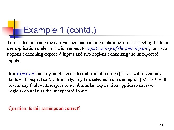
Example 1 (contd. ) Tests selected using the equivalence partitioning technique aim at targeting faults in the application under test with respect to inputs in any of the four regions, i. e. , two regions containing expected inputs and two regions containing the unexpected inputs. It is expected that any single test selected from the range [1. . 61] will reveal any fault with respect to R 1. Similarly, any test selected from the region [62. . 120] will reveal any fault with respect to R 2. A similar expectation applies to the two regions containing the unexpected inputs. Question: Is this assumption correct? 23

Example 2 This example shows a few ways to define equivalence classes based on the knowledge of requirements and the program text. Consider that word. Count method takes a word w and a filename f as input and returns the number of occurrences of w in the text contained in the file named f. An exception is raised if there is no file with name f. Using the partitioning method described in the previous example, we obtain the following equivalence classes. 24

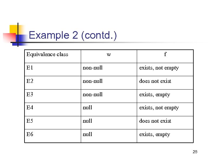
Example 2 (contd. ) Equivalence class w f E 1 non-null exists, not empty E 2 non-null does not exist E 3 non-null exists, empty E 4 null exists, not empty E 5 null does not exist E 6 null exists, empty 25

Example 2 (contd. ) Note that the number of equivalence classes without any knowledge of the program code is 2, whereas the number of equivalence classes on slide 25 is 6. An experienced tester will likely derive the six equivalence classes given above, and perhaps more, even before the code is available 26

Equivalence Classes based on Program Output In some cases the equivalence classes are based on the output generated by the program. For example, suppose that a program outputs an integer. It is worth asking: “Does the program ever generate a 0? What are the maximum and minimum possible values of the output? ” These two questions lead to two the following equivalence classes based on outputs: 27

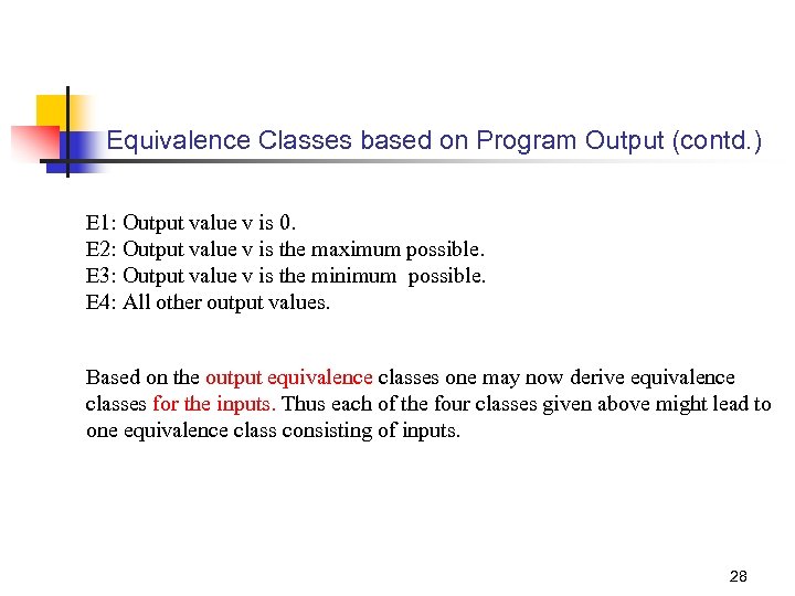
Equivalence Classes based on Program Output (contd. ) E 1: Output value v is 0. E 2: Output value v is the maximum possible. E 3: Output value v is the minimum possible. E 4: All other output values. Based on the output equivalence classes one may now derive equivalence classes for the inputs. Thus each of the four classes given above might lead to one equivalence class consisting of inputs. 28

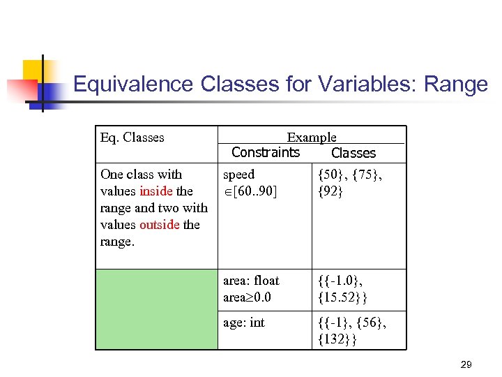
Equivalence Classes for Variables: Range Eq. Classes One class with values inside the range and two with values outside the range. Example Constraints Classes speed [60. . 90] {50}, {75}, {92} area: float area 0. 0 {{-1. 0}, {15. 52}} age: int {{-1}, {56}, {132}} 29

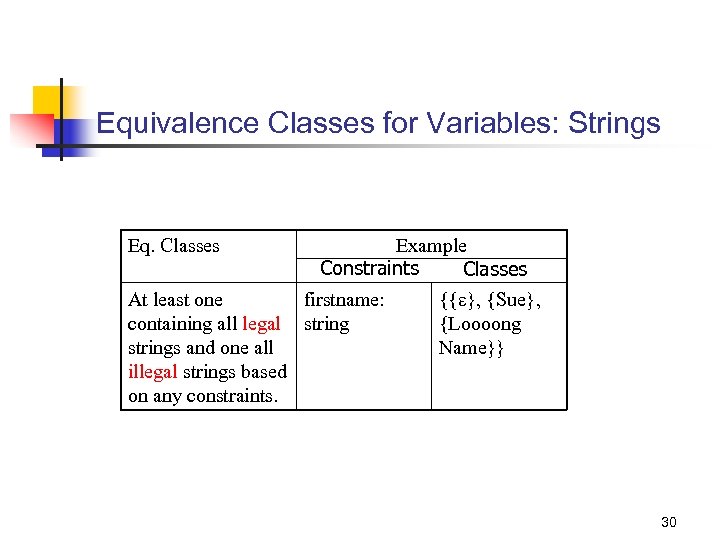
Equivalence Classes for Variables: Strings Eq. Classes At least one containing all legal strings and one all illegal strings based on any constraints. Example Constraints Classes firstname: {{ }, {Sue}, string {Loooong Name}} 30

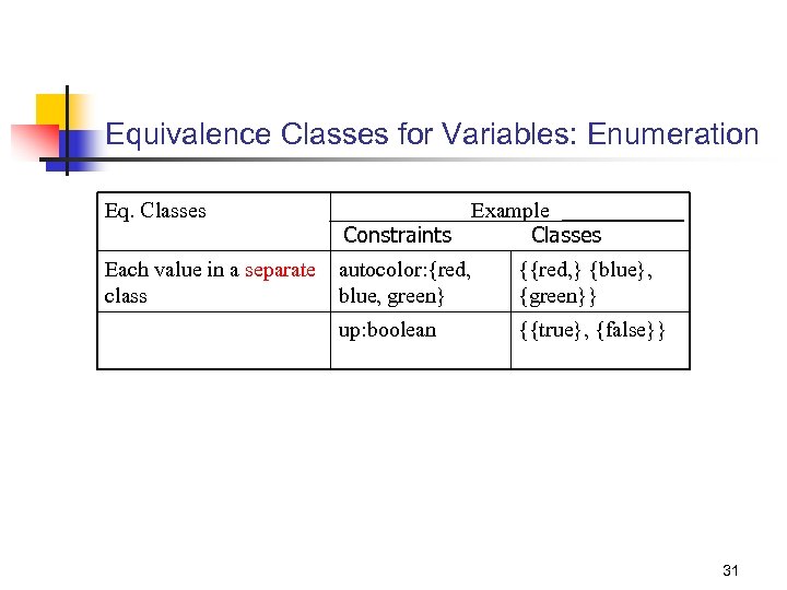
Equivalence Classes for Variables: Enumeration Eq. Classes Example Classes Constraints Each value in a separate class autocolor: {red, blue, green} {{red, } {blue}, {green}} up: boolean {{true}, {false}} 31

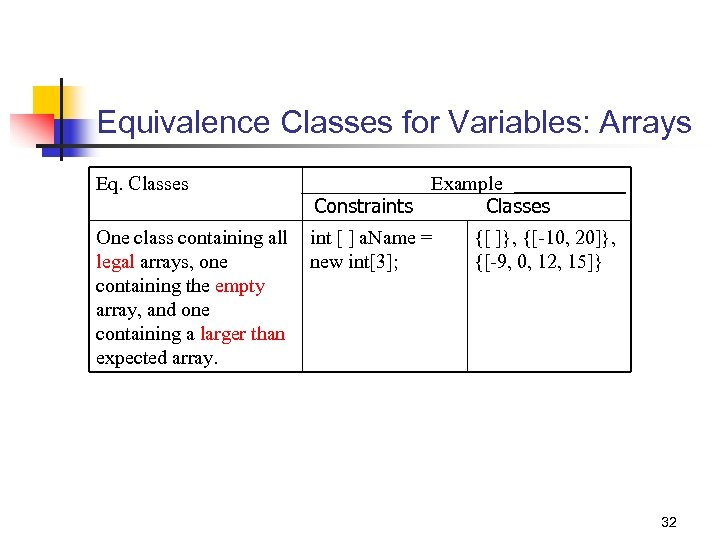
Equivalence Classes for Variables: Arrays Eq. Classes Example Classes Constraints One class containing all legal arrays, one containing the empty array, and one containing a larger than expected array. int [ ] a. Name = new int[3]; {[ ]}, {[-10, 20]}, {[-9, 0, 12, 15]} 32

Equivalence Classes for Variables: Compound Data Type Arrays in Java and structures in C++/C, are compound types. Such input types may arise while testing components of an application such as a function or an object. While generating equivalence classes for such inputs, one must consider legal and illegal values for each component of the structure. The next example illustrates the derivation of equivalence classes for an input variable that has a compound type. 33

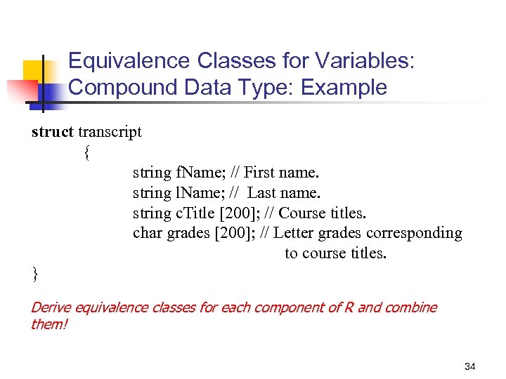
Equivalence Classes for Variables: Compound Data Type: Example struct transcript { string f. Name; // First name. string l. Name; // Last name. string c. Title [200]; // Course titles. char grades [200]; // Letter grades corresponding to course titles. } Derive equivalence classes for each component of R and combine them! 34

Unidimensional Partitioning One way to partition the input domain is to consider one input variable at a time. Thus each input variable leads to a partition of the input domain. We refer to this style of partitioning as unidimensional equivalence partitioning or simply unidimensional partitioning. This type of partitioning is commonly used. 35

Multidimensional Partitioning Another way is to consider the input domain I as the set product of the input variables and define a relation on I. This procedure creates one partition consisting of several equivalence classes. We refer to this method as multidimensional equivalence partitioning or simply multidimensional partitioning. Multidimensional partitioning leads to a large number of equivalence classes that are difficult to manage manually. Many classes so created might be infeasible. Nevertheless, equivalence classes so created offer an increased variety of tests as is illustrated in the next section. 36

Partitioning Example Consider an application that requires two integer inputs x and y. Each of these inputs is expected to lie in the following ranges: 3 x 7 and 5 y 9. For unidimensional partitioning we apply the partitioning guidelines to x and y individually. This leads to the following six equivalence classes. 37

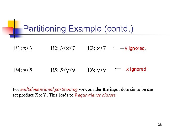
Partitioning Example (contd. ) E 1: x<3 E 2: 3 x 7 E 3: x>7 E 4: y<5 E 5: 5 y 9 E 6: y>9 y ignored. x ignored. For multidimensional partitioning we consider the input domain to be the set product X x Y. This leads to 9 equivalence classes 38

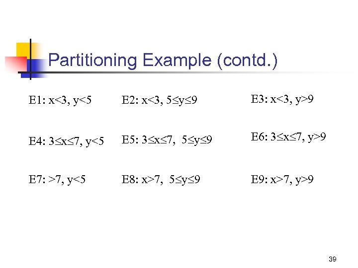
Partitioning Example (contd. ) E 1: x<3, y<5 E 2: x<3, 5 y 9 E 3: x<3, y>9 E 4: 3 x 7, y<5 E 5: 3 x 7, 5 y 9 E 6: 3 x 7, y>9 E 7: >7, y<5 E 8: x>7, 5 y 9 E 9: x>7, y>9 39

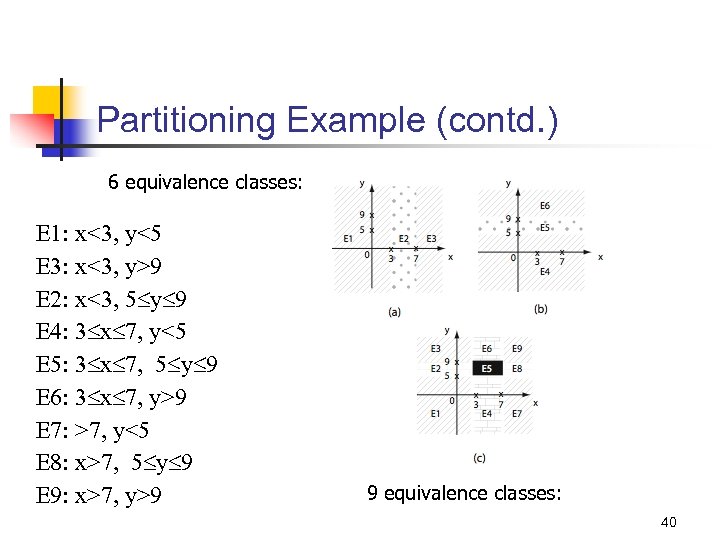
Partitioning Example (contd. ) 6 equivalence classes: E 1: x<3, y<5 E 3: x<3, y>9 E 2: x<3, 5 y 9 E 4: 3 x 7, y<5 E 5: 3 x 7, 5 y 9 E 6: 3 x 7, y>9 E 7: >7, y<5 E 8: x>7, 5 y 9 E 9: x>7, y>9 9 equivalence classes: 40

Systematic Procedure for Equivalence Partitioning 1. Identify the input domain: Read the requirements carefully and identify all input and output variables, their types, and any conditions associated with their use. Environment variables, such as class variables used in the method under test and environment variables in Unix, Windows, and other operating systems, also serve as input variables. Given the set of values each variable can assume, an approximation to the input domain is the product of these sets. 41

Systematic Procedure for Equivalence Partitioning (contd. ) 2. Equivalence classing: Partition the set of values of each variable into disjoint subsets. Each subset is an equivalence class. Values for which the program is expected to behave in the “same way” are grouped together. Note that “same way” needs to be defined by the tester. 42

Systematic Procedure for Equivalence Partitioning (contd. ) 3. Combine equivalence classes: This step is usually omitted and the equivalence classes defined for each variable are directly used to select test cases. However, by not combining the equivalence classes, one misses the opportunity to generate useful tests. The equivalence classes are combined using the multidimensional partitioning approach described earlier. 43

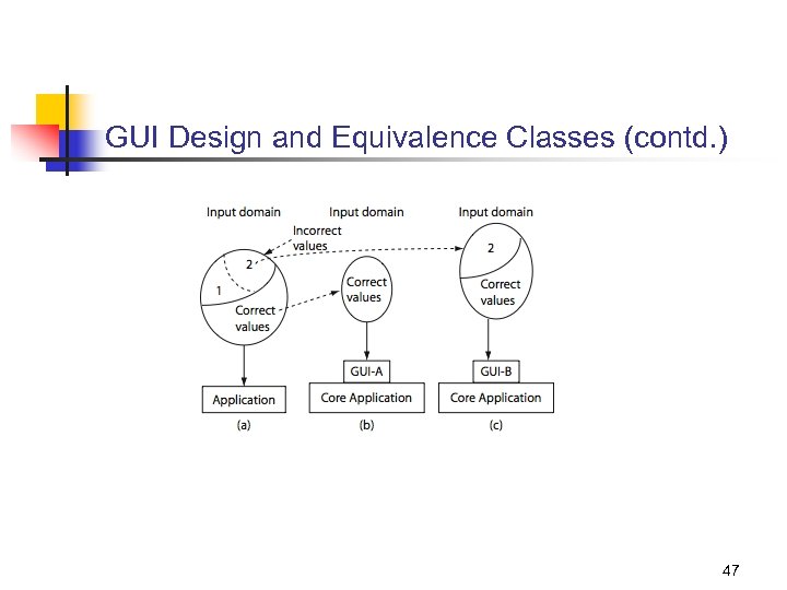
Systematic Procedure for Equivalence Partitioning (contd. ) 4. Identify infeasible equivalence classes: An infeasible equivalence class is one that contains a combination of input data that cannot be generated during test. Such an equivalence class might arise due to several reasons. For example, suppose that an application is tested via its GUI, i. e. , data is input using commands available in the GUI. The GUI might disallow invalid inputs by offering a palette of valid inputs only. There might also be constraints in the requirements that render certain equivalence infeasible. 44

GUI Design and Equivalence Classes While designing equivalence classes for programs that obtain input exclusively from a keyboard, one must account for the possibility of errors in data entry. Example: An application places a constraint on an input variable x such that it can assume integral values in the range 3. . 7. However, testing must account for the possibility that a user may inadvertently enter a value for x that is out of range. 45

GUI Design and Equivalence Classes (contd. ) Suppose that all data entry to the application is via a GUI front end. Suppose also that the GUI offers exactly five correct choices to the user for x. In such a situation it is impossible to test the application with a value of x that is out of range. Hence only the correct values of x will be input. See figures on the next slide. 46

GUI Design and Equivalence Classes (contd. ) 47

Boundary Value Analysis 48

Errors at the Boundaries Experience indicates that programmers make mistakes in processing values at and near the boundaries of equivalence classes. For example, suppose that method M is required to compute a function f 1 when x 0 is true and function f 2 otherwise. However, M has an error due to which it computes f 1 for x <0 and f 2 otherwise. Obviously, this fault can be revealed when M is tested against x = 0, but not if the input test set is, for example, {-4, 7} derived using equivalence partitioning. In this example, the value x=0, lies at the boundary of the equivalence classes x 0 and x>0. 49

Boundary Value Analysis (BVA) Boundary value analysis is a test selection technique that targets faults in applications at the boundaries of equivalence classes. While equivalence partitioning selects tests from within equivalence classes, boundary value analysis focuses on tests at and near the boundaries of equivalence classes. Certainly, tests derived using either of the two techniques may overlap. 50

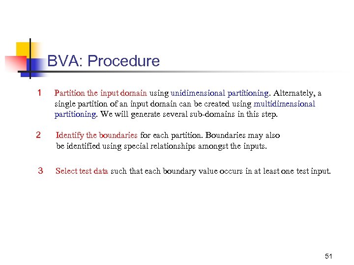
BVA: Procedure 1 Partition the input domain using unidimensional partitioning. Alternately, a single partition of an input domain can be created using multidimensional partitioning. We will generate several sub-domains in this step. 2 Identify the boundaries for each partition. Boundaries may also be identified using special relationships amongst the inputs. 3 Select test data such that each boundary value occurs in at least one test input. 51

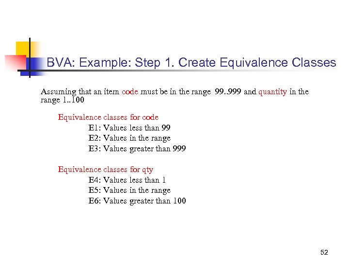
BVA: Example: Step 1. Create Equivalence Classes Assuming that an item code must be in the range 99. . 999 and quantity in the range 1. . 100 Equivalence classes for code E 1: Values less than 99 E 2: Values in the range E 3: Values greater than 999 Equivalence classes for qty E 4: Values less than 1 E 5: Values in the range E 6: Values greater than 100 52

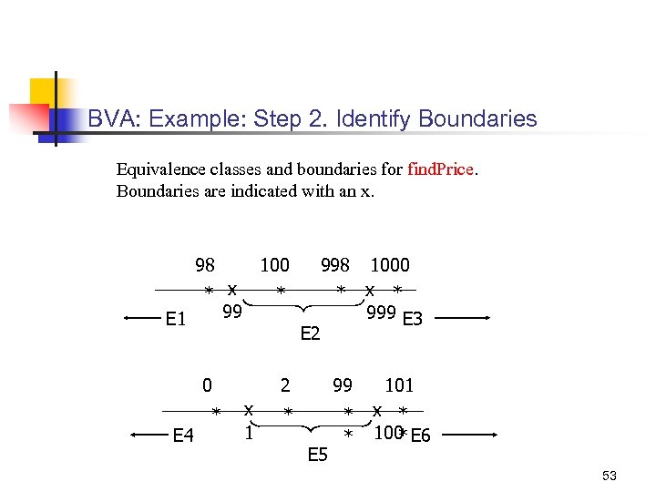
BVA: Example: Step 2. Identify Boundaries Equivalence classes and boundaries for find. Price. Boundaries are indicated with an x. 98 100 998 * x 99 E 1 * * 0 2 99 * * * E 4 * E 2 x 1 E 5 1000 x * 999 E 3 101 x * 100 E 6 * 53

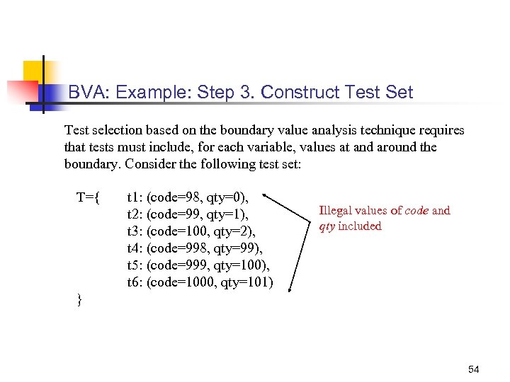
BVA: Example: Step 3. Construct Test Set Test selection based on the boundary value analysis technique requires that tests must include, for each variable, values at and around the boundary. Consider the following test set: T={ t 1: (code=98, qty=0), t 2: (code=99, qty=1), t 3: (code=100, qty=2), t 4: (code=998, qty=99), t 5: (code=999, qty=100), t 6: (code=1000, qty=101) Illegal values of code and qty included } 54

Testing Predicates 55

Test Generation from Predicates (1) We will now examine three techniques, named BOR (Boolean Operator), BRO (Boolean and Relational Operator), and BRE (Boolean Relational Expression) for generating tests that are guaranteed to detect certain faults in the coding of conditions. The conditions from which tests are generated might arise from requirements or might be embedded in the program to be tested. Conditions guard actions. For example, if condition then action is a typical format of many functional requirements. 56

Test Generation from Predicates (2) A condition is represented formally as a predicate, also known as a Boolean expression. For example, consider the requirement “if the printer is ON and has paper then send document to printer. ” This statement consists of a condition part and an action part. The following predicate represents the condition part of the statement pr: (printerstatus = ON) (printertray = empty) 57

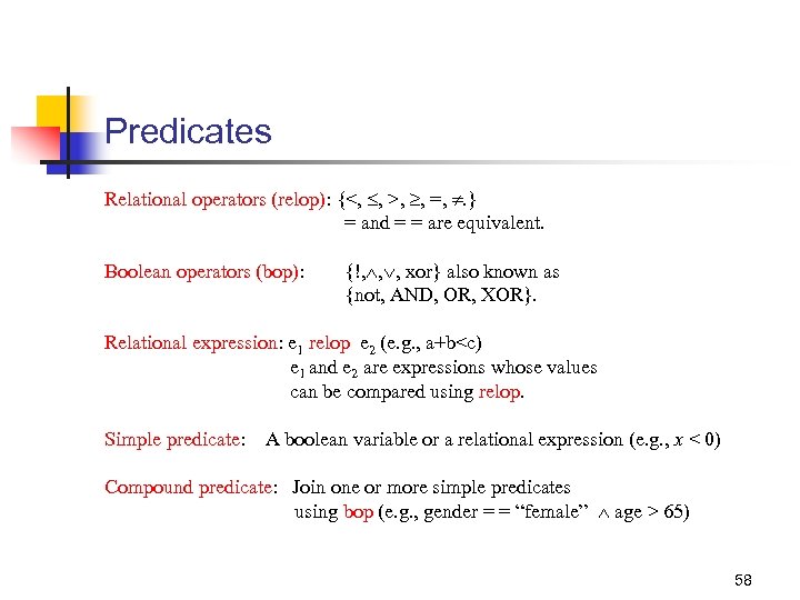
Predicates Relational operators (relop): {<, , >, , =, . } = and = = are equivalent. Boolean operators (bop): {!, , , xor} also known as {not, AND, OR, XOR}. Relational expression: e 1 relop e 2 (e. g. , a+b<c) e 1 and e 2 are expressions whose values can be compared using relop. Simple predicate: A boolean variable or a relational expression (e. g. , x < 0) Compound predicate: Join one or more simple predicates using bop (e. g. , gender = = “female” age > 65) 58

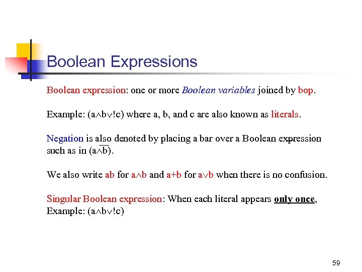
Boolean Expressions Boolean expression: one or more Boolean variables joined by bop. Example: (a b !c) where a, b, and c are also known as literals. Negation is also denoted by placing a bar over a Boolean expression such as in (a b). We also write ab for a b and a+b for a b when there is no confusion. Singular Boolean expression: When each literal appears only once, Example: (a b !c) 59

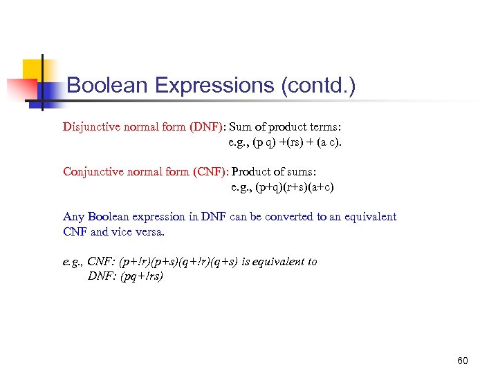
Boolean Expressions (contd. ) Disjunctive normal form (DNF): Sum of product terms: e. g. , (p q) +(rs) + (a c). Conjunctive normal form (CNF): Product of sums: e. g. , (p+q)(r+s)(a+c) Any Boolean expression in DNF can be converted to an equivalent CNF and vice versa. e. g. , CNF: (p+!r)(p+s)(q+!r)(q+s) is equivalent to DNF: (pq+!rs) 60

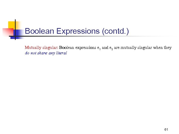
Boolean Expressions (contd. ) Mutually singular: Boolean expressions e 1 and e 2 are mutually singular when they do not share any literal 61

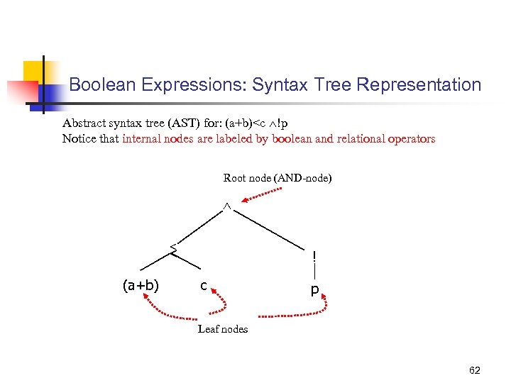
Boolean Expressions: Syntax Tree Representation Abstract syntax tree (AST) for: (a+b)<c !p Notice that internal nodes are labeled by boolean and relational operators Root node (AND-node) < < (a+b) ! c p Leaf nodes 62

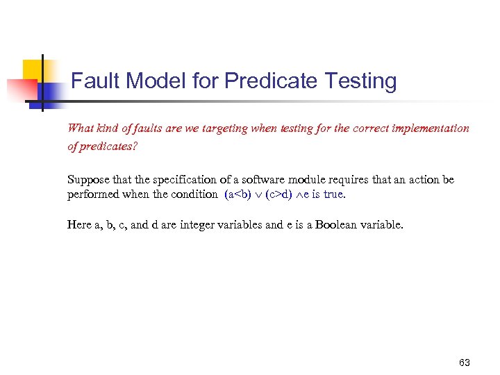
Fault Model for Predicate Testing What kind of faults are we targeting when testing for the correct implementation of predicates? Suppose that the specification of a software module requires that an action be performed when the condition (a<b) (c>d) e is true. Here a, b, c, and d are integer variables and e is a Boolean variable. 63

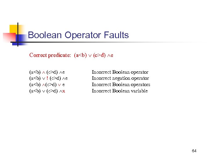
Boolean Operator Faults Correct predicate: (a<b) (c>d) e (a<b) ! (c>d) e (a<b) (c>d) e (a<b) (c>d) x Incorrect Boolean operator Incorrect negation operator Incorrect Boolean operators Incorrect Boolean variable 64

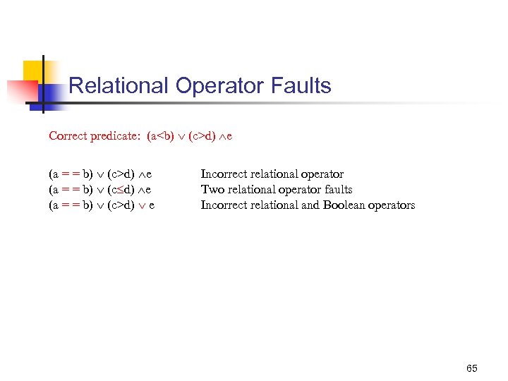
Relational Operator Faults Correct predicate: (a<b) (c>d) e (a = = b) (c>d) e Incorrect relational operator Two relational operator faults Incorrect relational and Boolean operators 65

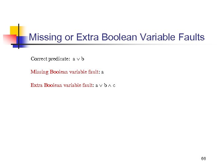
Missing or Extra Boolean Variable Faults Correct predicate: a b Missing Boolean variable fault: a Extra Boolean variable fault: a b c 66

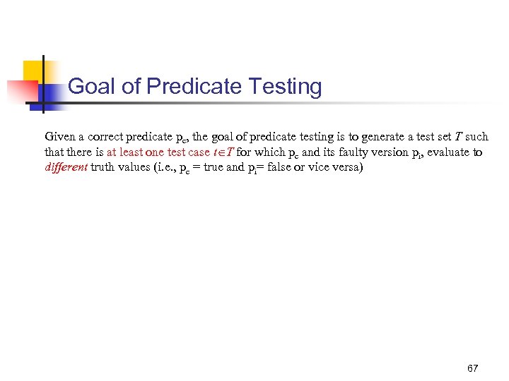
Goal of Predicate Testing Given a correct predicate pc, the goal of predicate testing is to generate a test set T such that there is at least one test case t T for which pc and its faulty version pi, evaluate to different truth values (i. e. , pc = true and pi= false or vice versa) 67

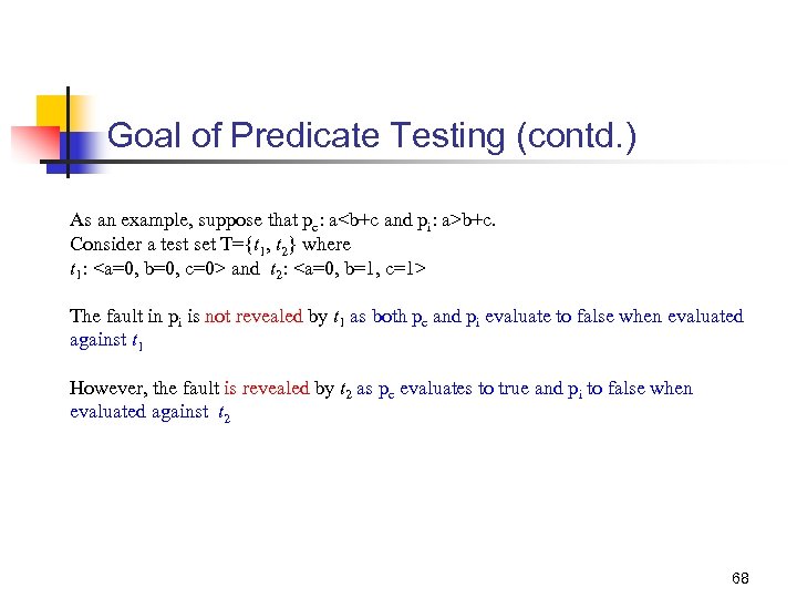
Goal of Predicate Testing (contd. ) As an example, suppose that pc: a<b+c and pi: a>b+c. Consider a test set T={t 1, t 2} where t 1: <a=0, b=0, c=0> and t 2: <a=0, b=1, c=1> The fault in pi is not revealed by t 1 as both pc and pi evaluate to false when evaluated against t 1 However, the fault is revealed by t 2 as pc evaluates to true and pi to false when evaluated against t 2 68

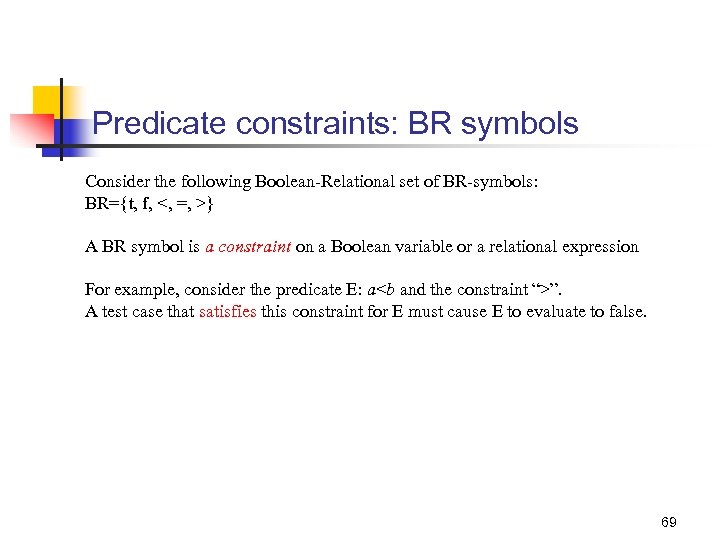
Predicate constraints: BR symbols Consider the following Boolean-Relational set of BR-symbols: BR={t, f, <, =, >} A BR symbol is a constraint on a Boolean variable or a relational expression For example, consider the predicate E: a”. A test case that satisfies this constraint for E must cause E to evaluate to false. 69

Infeasible Constraints A constraint C is considered infeasible for predicate pr if there exists no input values for the variables in pr that satisfy C. For example, the constraint t (true) is infeasible for the predicate (a>b) (b>d) if it is known that d>a 70

Predicate Constraints Let pr denote a predicate with n, n>0, and operators. A predicate constraint C for predicate pr is a sequence of (n+1) BR symbols, one for each Boolean variable or relational expression in pr. When clear from context, we refer to “predicate constraint” as simply constraint. Test case t satisfies C for predicate pr, if each component of pr satisfies the corresponding constraint in C when evaluated against t. Constraint C for predicate pr guides the development of a test for pr, i. e. , it offers hints on what the values of the variables should be for pr to satisfy C. 71

Predicate Constraints: Example Consider the predicate pr: b (r<s) (u v) and a constraint C: (t, =, >) The following test case satisfies C for pr <b=true, r=1, s=1, u=1, v=0> The following test case does not satisfy C for pr <b=true, r=1, s=2, u=1, v=2> 72

True and False Constraints pr(C) denotes the value of predicate pr evaluated using a test case that satisfies C C is referred to as a true constraint when pr(C) is true and a false constraint otherwise A set of constraints S is partitioned into subsets St and Sf, respectively, such that for each C in St, pr(C) =true, and for any C in Sf, pr(C) =false. S= St Sf 73

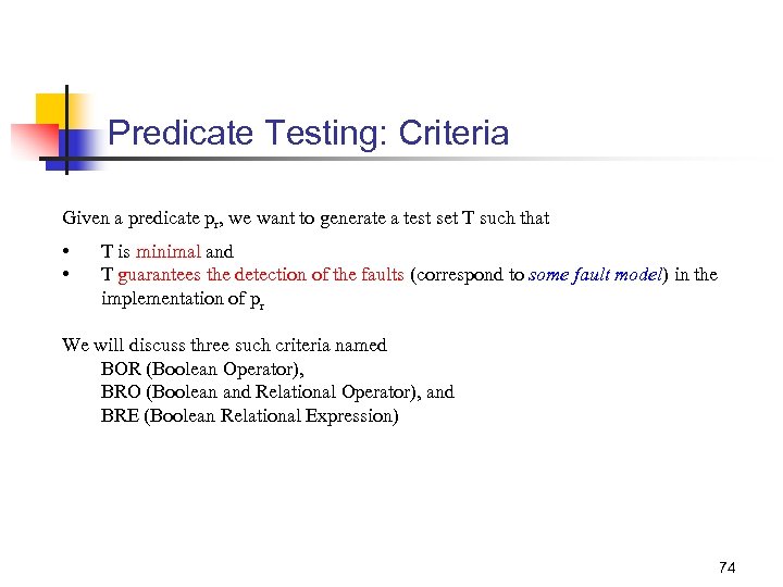
Predicate Testing: Criteria Given a predicate pr, we want to generate a test set T such that • • T is minimal and T guarantees the detection of the faults (correspond to some fault model) in the implementation of pr We will discuss three such criteria named BOR (Boolean Operator), BRO (Boolean and Relational Operator), and BRE (Boolean Relational Expression) 74

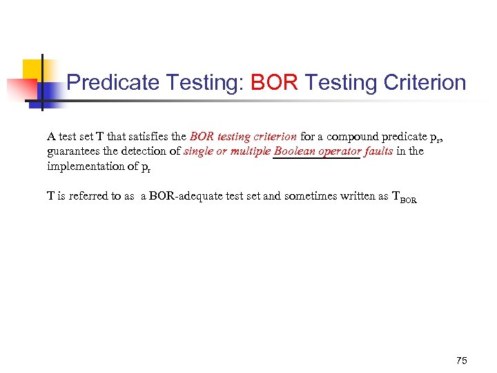
Predicate Testing: BOR Testing Criterion A test set T that satisfies the BOR testing criterion for a compound predicate pr, guarantees the detection of single or multiple Boolean operator faults in the implementation of pr T is referred to as a BOR-adequate test set and sometimes written as TBOR 75

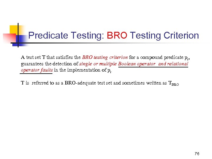
Predicate Testing: BRO Testing Criterion A test set T that satisfies the BRO testing criterion for a compound predicate pr, guarantees the detection of single or multiple Boolean operator and relational operator faults in the implementation of pr T is referred to as a BRO-adequate test set and sometimes written as TBRO 76

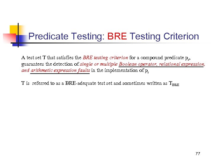
Predicate Testing: BRE Testing Criterion A test set T that satisfies the BRE testing criterion for a compound predicate pr, guarantees the detection of single or multiple Boolean operator, relational expression, and arithmetic expression faults in the implementation of pr T is referred to as a BRE-adequate test set and sometimes written as T BRE 77

Predicate Testing: Guaranteeing Fault Detection Let Tx, x {BOR, BRO, BRE}, be a test set derived from predicate pr Let pf be another predicate obtained from pr by injecting single or multiple faults of one of three kinds: Boolean operator fault, relational operator fault, and arithmetic expression fault Tx is said to guarantee the detection of faults in pf if for some t Tx, pr(t)≠ pf(t) 78

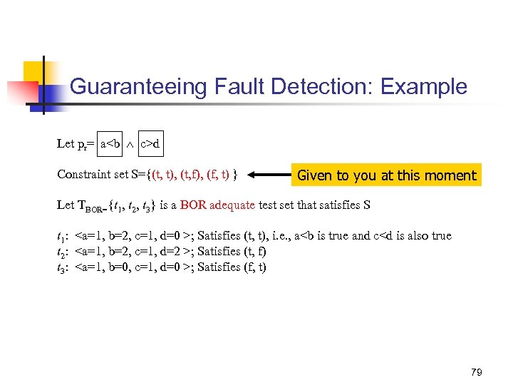
Guaranteeing Fault Detection: Example Let pr= ad Constraint set S={(t, t), (t, f), (f, t) } Given to you at this moment Let TBOR={t 1, t 2, t 3} is a BOR adequate test set that satisfies S t 1: <a=1, b=2, c=1, d=0 >; Satisfies (t, t), i. e. , a; Satisfies (t, f) t 3: <a=1, b=0, c=1, d=0 >; Satisfies (f, t) 79

Guaranteeing Fault Detection: In Class Exercise (1) Inject single or multiple Boolean operator faults in pr: ad and show that T guarantees the detection of each fault. 80

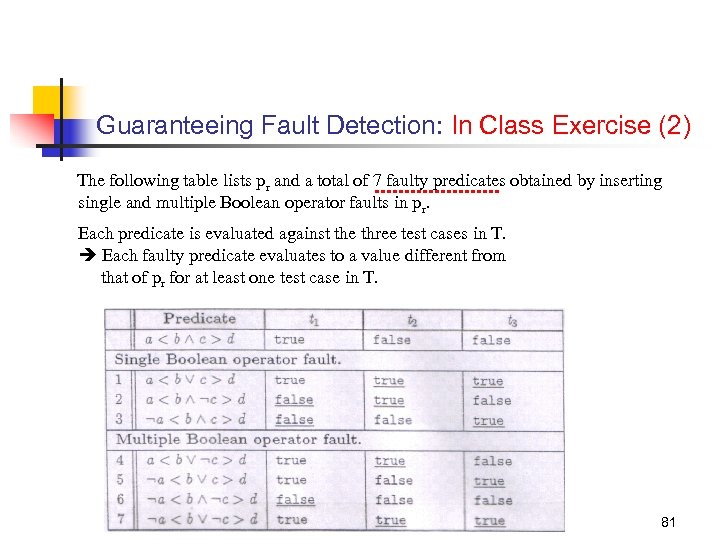
Guaranteeing Fault Detection: In Class Exercise (2) The following table lists pr and a total of 7 faulty predicates obtained by inserting single and multiple Boolean operator faults in pr. Each predicate is evaluated against the three test cases in T. Each faulty predicate evaluates to a value different from that of pr for at least one test case in T. 81

Guaranteeing Fault Detection: In Class Exercise (3) Can we delete any of these three test cases in T and still guarantee the detection of all the Boolean operator faults? 82

Guaranteeing Fault Detection: In Class Exercise (4) Suppose we remove t 2, then the faulty predicate 4 in the previous table cannot be distinguished from pr by tests t 1 and t 3 In fact, if we remove t 2 from T, then T is no longer BOR adequate because of the constraints (t, f) is not satisfied We can verify that if any column in the previous table is removed, at least one of the faulty predicates will be left indistinguishable by the tests in the remaining two columns 83

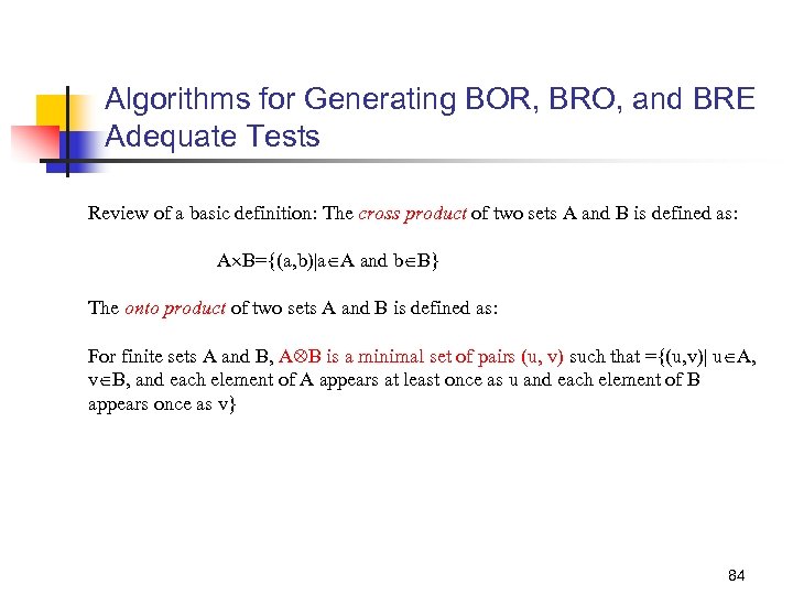
Algorithms for Generating BOR, BRO, and BRE Adequate Tests Review of a basic definition: The cross product of two sets A and B is defined as: A B={(a, b)|a A and b B} The onto product of two sets A and B is defined as: For finite sets A and B, A B is a minimal set of pairs (u, v) such that ={(u, v)| u A, v B, and each element of A appears at least once as u and each element of B appears once as v} 84

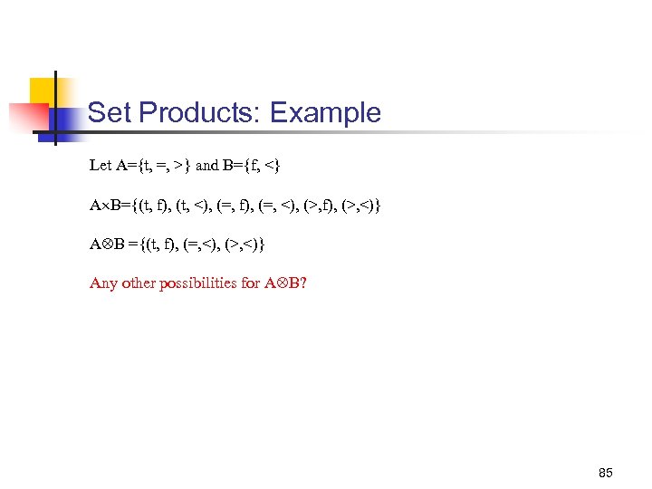
Set Products: Example Let A={t, =, >} and B={f, <} A B={(t, f), (t, <), (=, f), (=, <), (>, f), (>, <)} A B ={(t, f), (=, <), (>, <)} Any other possibilities for A B? 85

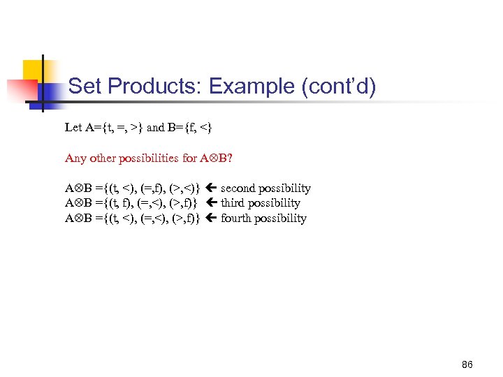
Set Products: Example (cont’d) Let A={t, =, >} and B={f, <} Any other possibilities for A B? A B ={(t, <), (=, f), (>, <)} second possibility A B ={(t, f), (=, <), (>, f)} third possibility A B ={(t, <), (=, <), (>, f)} fourth possibility 86

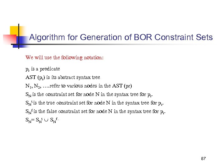
Algorithm for Generation of BOR Constraint Sets We will use the following notation: pr is a predicate AST (pr) is its abstract syntax tree N 1, N 2, …. refer to various nodes in the AST (pr) SN is the constraint set for node N in the syntax tree for pr. SNt is the true constraint set for node N in the syntax tree for pr. SNf is the false constraint set for node N in the syntax tree for pr. SN = S N t SN f. 87

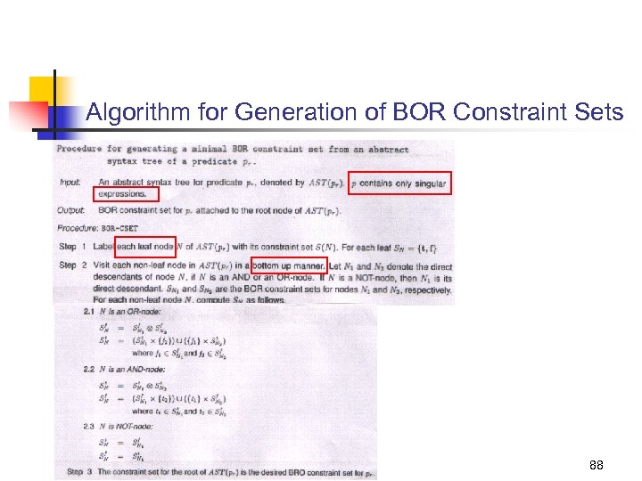
Algorithm for Generation of BOR Constraint Sets 88

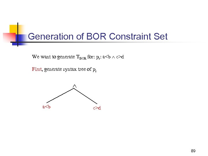
Generation of BOR Constraint Set We want to generate TBOR for: pr: ad First, generate syntax tree of pr ad 89

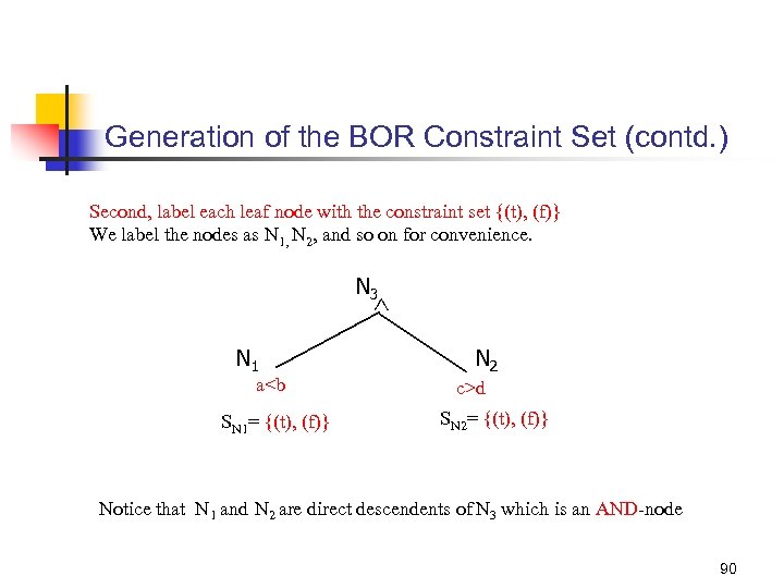
Generation of the BOR Constraint Set (contd. ) Second, label each leaf node with the constraint set {(t), (f)} We label the nodes as N 1, N 2, and so on for convenience. N 3 N 1 ad SN 2= {(t), (f)} Notice that N 1 and N 2 are direct descendents of N 3 which is an AND-node 90

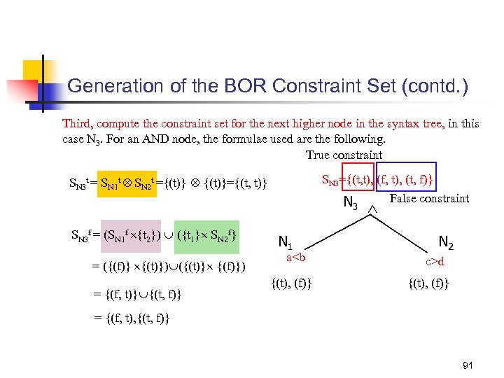
Generation of the BOR Constraint Set (contd. ) Third, compute the constraint set for the next higher node in the syntax tree, in this case N 3. For an AND node, the formulae used are the following. True constraint SN 3={(t, t), (f, t), (t, f)} False constraint N SN 3 t = SN 1 t SN 2 t ={(t)} {(t)}={(t, t)} 3 SN 3 f = (SN 1 f {t 2}) ({t 1} SN 2 f} = ({(f)} {(t)}) ({(t)} {(f)}) = {(f, t)} {(t, f)} N 1 ad {(t), (f)} = {(f, t), {(t, f)} 91

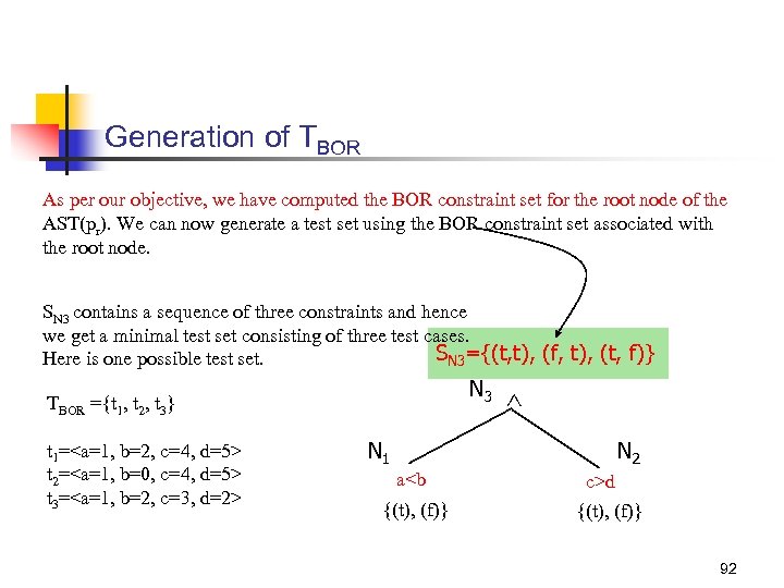
Generation of TBOR As per our objective, we have computed the BOR constraint set for the root node of the AST(pr). We can now generate a test set using the BOR constraint set associated with the root node. SN 3 contains a sequence of three constraints and hence we get a minimal test set consisting of three test cases. SN 3={(t, t), (f, t), (t, f)} Here is one possible test set. N 3 TBOR ={t 1, t 2, t 3} t 1=<a=1, b=2, c=4, d=5> t 2=<a=1, b=0, c=4, d=5> t 3=<a=1, b=2, c=3, d=2> N 2 N 1 ad {(t), (f)} 92

Another Example for TBOR (1) Generate the BOR-constraint sets for the predicate (a+b)<c !p (r > s) 93

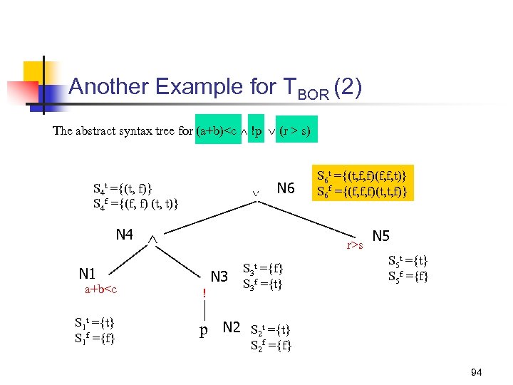
Another Example for TBOR (2) The abstract syntax tree for (a+b)<c !p (r > s) N 6 S 4 t ={(t, f)} S 4 f ={(f, f) (t, t)} N 4 r>s N 1 a+b<c S 1 t ={t} S 1 f ={f} S 6 t ={(t, f, f)(f, f, t)} S 6 f ={(f, f, f)(t, t, f)} N 3 ! p N 2 S 3 ={f} S 3 f ={t} t N 5 S 5 t ={t} S 5 f ={f} S 2 t ={t} S 2 f ={f} 94

Generation of BRO Constraint Set Recall that a test set adequate with respect to a BRO constraint set for predicate p r, guarantees the detection of all combinations of single or multiple Boolean operator and relational operator faults. 95

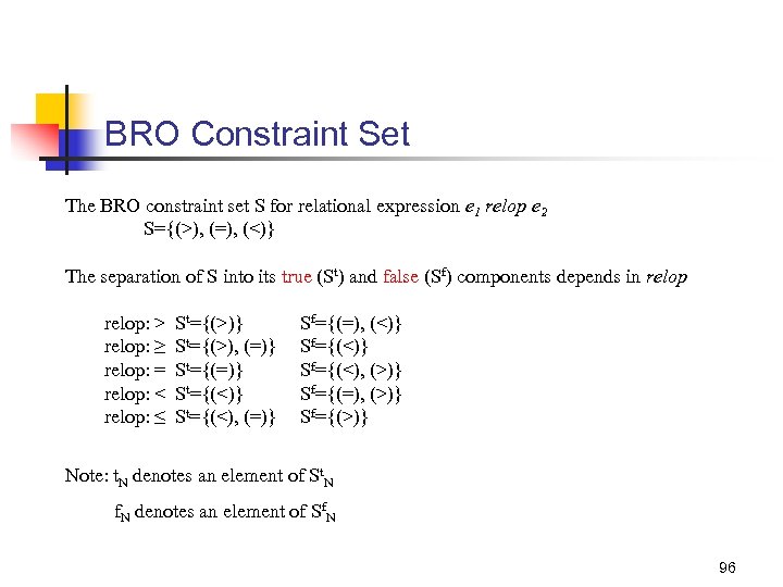
BRO Constraint Set The BRO constraint set S for relational expression e 1 relop e 2 S={(>), (=), (<)} The separation of S into its true (St) and false (Sf) components depends in relop: > relop: ≥ relop: = relop: < relop: ≤ St={(>)} St={(>), (=)} St={(<)} St={(<), (=)} Sf={(=), (<)} Sf={(<), (>)} Sf={(=), (>)} Sf={(>)} Note: t. N denotes an element of St. N f. N denotes an element of Sf. N 96

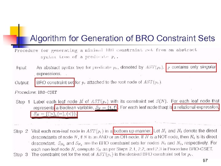
Algorithm for Generation of BRO Constraint Sets 97

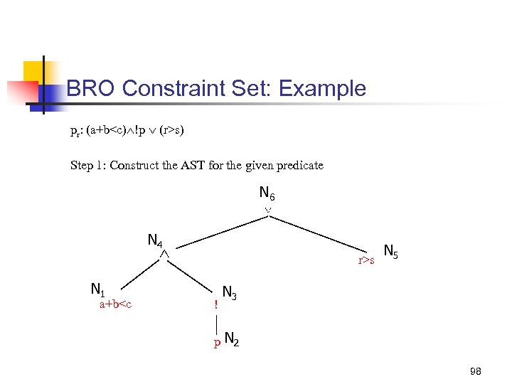
BRO Constraint Set: Example pr: (a+b<c) !p (r>s) Step 1: Construct the AST for the given predicate N 6 N 4 N 1 a+b<c r>s ! N 5 N 3 p N 2 98

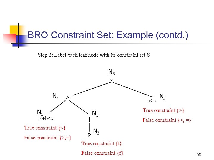
BRO Constraint Set: Example (contd. ) Step 2: Label each leaf node with its constraint set S N 6 N 4 N 1 a+b<c True constraint {<} False constraint {>, =} r>s ! N 3 N 5 True constraint {>} False constraint {<, =} p N 2 True constraint {t} False constraint {f} 99

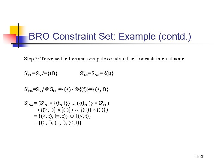
BRO Constraint Set: Example (contd. ) Step 2: Traverse the tree and compute constraint set for each internal node St. N 3=SN 2 f={(f)} Sf. N 3=SN 2 t= {(t)} St. N 4=SN 1 t SN 3 t={(<)} {(f)}={(<, f)} Sf. N 4 = (Sf. N 1 {(t. N 3)}) ({(t. N 1)} Sf. N 3) = ({(>, =)} {(f)}) {(<)} {(t)}) = {(>, f), (=, f)} {(<, t)} = {(>, f), (=, f), (<, t)} 100

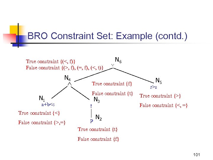
BRO Constraint Set: Example (contd. ) True constraint {(<, f)} False constraint {(>, f), (=, f), (<, t)} N 4 N 1 a+b<c True constraint {<} False constraint {>, =} N 6 True constraint {f} False constraint {t} ! N 3 N 5 r>s True constraint {>} False constraint {<, =} p N 2 True constraint {t} False constraint {f} 101

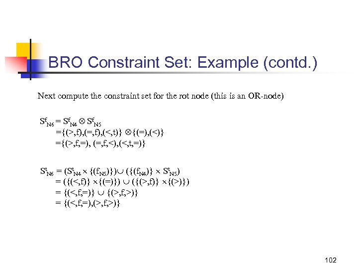
BRO Constraint Set: Example (contd. ) Next compute the constraint set for the rot node (this is an OR-node) Sf. N 6 = Sf. N 4 Sf. N 5 ={(>, f), (=, f), (<, t)} {(=), (<)} ={(>, f, =), (=, f, <), (<, t, =)} St. N 6 = (St. N 4 {(f. N 5)}) ({(f. N 4)} St. N 5) = ({(<, f)} {(=)}) ({(>, f)} {(>)}) = {(<, f, =)} {(>, f, >)} = {(<, f, =), (>, f, >)} 102

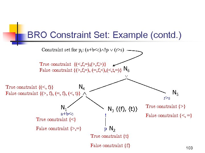
BRO Constraint Set: Example (contd. ) Constraint set for pr: (a+b<c) !p (r>s) True constraint {(<, f, =), (>, f, >)} False constraint {(>, f, =), (=, f, <), (<, t, =)} N 6 True constraint {(<, f)} N 4 False constraint {(>, f), (=, f), (<, t)} r>s N 1 a+b<c True constraint {<} False constraint {>, =} ! N 3 {(f), {t)} N 5 True constraint {>} False constraint {<, =} p N 2 True constraint {t} False constraint {f} 103

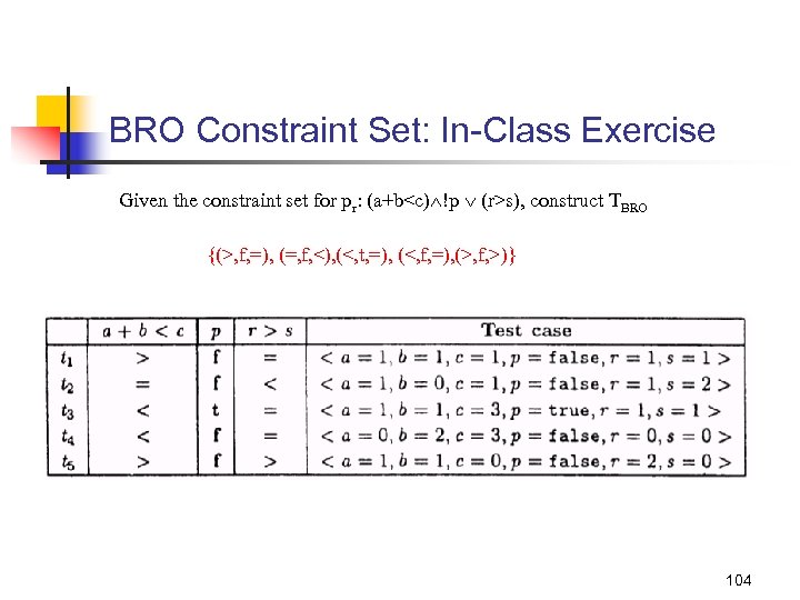
BRO Constraint Set: In-Class Exercise Given the constraint set for pr: (a+b<c) !p (r>s), construct TBRO {(>, f, =), (=, f, <), (<, t, =), (<, f, =), (>, f, >)} 104

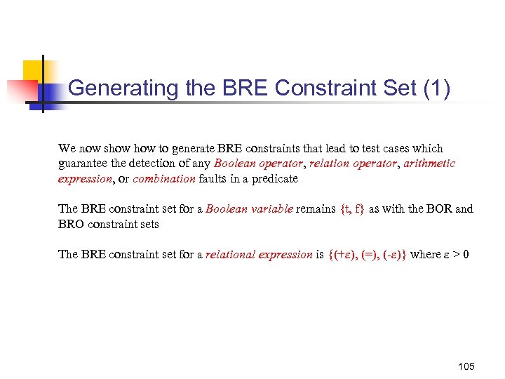
Generating the BRE Constraint Set (1) We now show to generate BRE constraints that lead to test cases which guarantee the detection of any Boolean operator, relation operator, arithmetic expression, or combination faults in a predicate The BRE constraint set for a Boolean variable remains {t, f} as with the BOR and BRO constraint sets The BRE constraint set for a relational expression is {(+ ), (=), (- )} where > 0 105

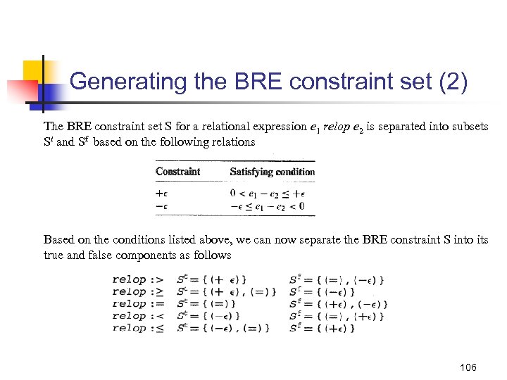
Generating the BRE constraint set (2) The BRE constraint set S for a relational expression e 1 relop e 2 is separated into subsets St and Sf based on the following relations Based on the conditions listed above, we can now separate the BRE constraint S into its true and false components as follows 106

Algorithm for Generation of BRE constraint sets (1) The procedure to generate a minimal BRE-constraint set is similar to that for BRO and BOR. The only difference lies in the construction of the constraint sets for the leaves. 107

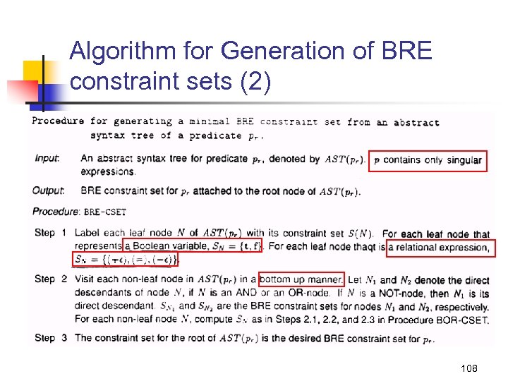
Algorithm for Generation of BRE constraint sets (2) 108

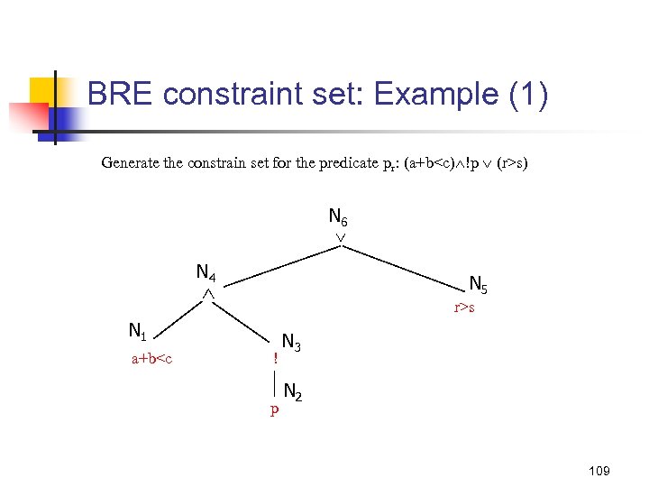
BRE constraint set: Example (1) Generate the constrain set for the predicate pr: (a+b<c) !p (r>s) N 6 N 4 N 5 r>s N 1 a+b<c ! p N 3 N 2 109

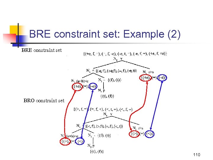
BRE constraint set: Example (2) BRE constraint set BRO constraint set 110

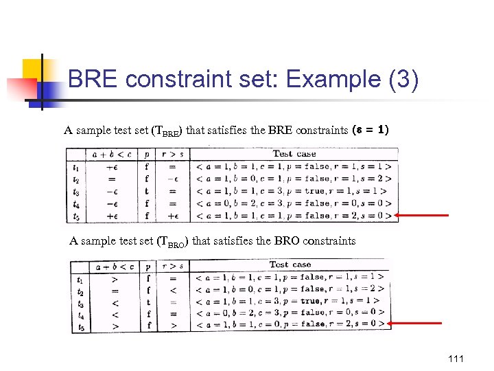
BRE constraint set: Example (3) A sample test set (TBRE) that satisfies the BRE constraints (e = 1) A sample test set (TBRO) that satisfies the BRO constraints 111

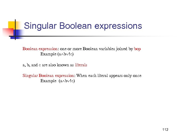
Singular Boolean expressions Boolean expression: one or more Boolean variables joined by bop Example (a b !c) a, b, and c are also known as literals Singular Boolean expression: When each literal appears only once Example (a b !c) 112

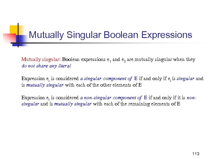
Mutually Singular Boolean Expressions Mutually singular: Boolean expressions e 1 and e 2 are mutually singular when they do not share any literal Expression ei is considered a singular component of E if and only if ei is singular and is mutually singular with each of the other elements of E Expression ei is considered a non-singular component of E if and only if it is nonsingular and is mutually singular with each of the remaining elements of E 113

BOR constraints for non-singular expressions Test generation procedures described so far are for singular predicates. Recall that a singular predicate contains only one occurrence of each variable We will now learn how to generate BOR constraints for non-singular predicates First, let us look at some non-singular expressions, their respective disjunctive normal forms (DNF), and their mutually singular components 114

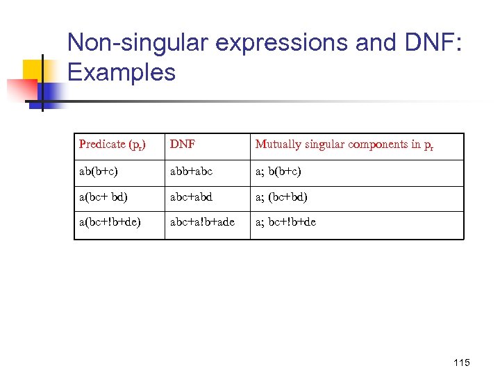
Non-singular expressions and DNF: Examples Predicate (pr) DNF Mutually singular components in pr ab(b+c) abb+abc a; b(b+c) a(bc+ bd) abc+abd a; (bc+bd) a(bc+!b+de) abc+a!b+ade a; bc+!b+de 115

Generating BOR constraints for nonsingular expressions We proceed in two steps: First we will examine the Meaning Impact (MI) procedure for generating a minimal set of constraints from a possibly non-singular predicate Next, we will examine the procedure to generate BOR constraint set for a non-singular predicate 116

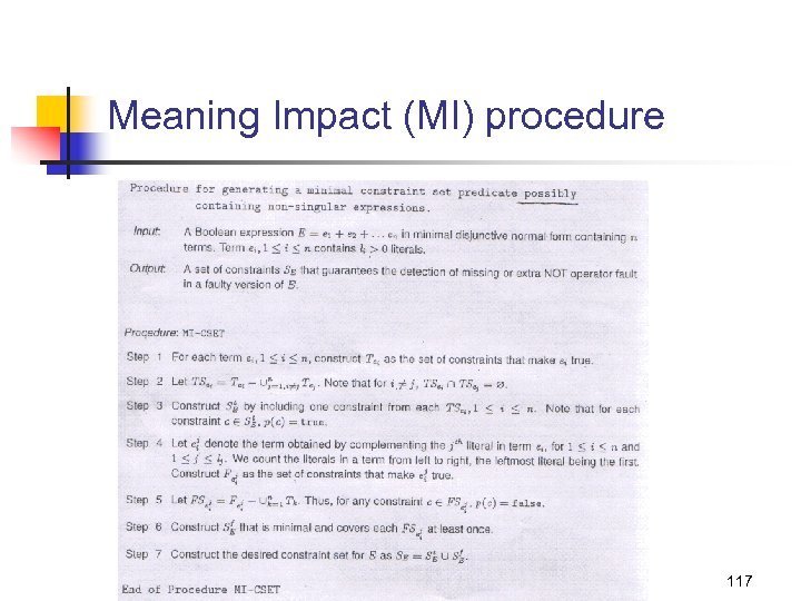
Meaning Impact (MI) procedure 117

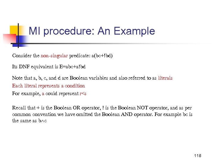
MI procedure: An Example Consider the non-singular predicate: a(bc+!bd) Its DNF equivalent is E=abc+a!bd Note that a, b, c, and d are Boolean variables and also referred to as literals Each literal represents a condition For example, a could represent r<s Recall that + is the Boolean OR operator, ! is the Boolean NOT operator, and as per common convention we have omitted the Boolean AND operator. For example bc is the same as b c 118

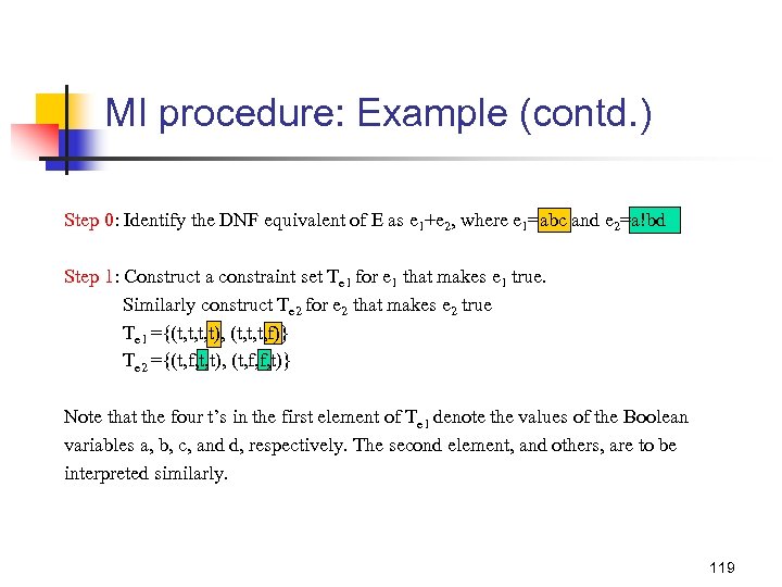
MI procedure: Example (contd. ) Step 0: Identify the DNF equivalent of E as e 1+e 2, where e 1=abc and e 2=a!bd Step 1: Construct a constraint set Te 1 for e 1 that makes e 1 true. Similarly construct Te 2 for e 2 that makes e 2 true Te 1 ={(t, t, t, t), (t, t, t, f)} Te 2 ={(t, f, t, t), (t, f, f, t)} Note that the four t’s in the first element of Te 1 denote the values of the Boolean variables a, b, c, and d, respectively. The second element, and others, are to be interpreted similarly. 119

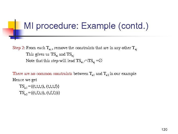
MI procedure: Example (contd. ) Step 2: From each Tei , remove the constraints that are in any other Tej This gives us TSei and TSej Note that this step will lead TSei TSej = There are no common constraints between Te 1 and Te 2 in our example Hence we get TSe 1 ={(t, t, t, t), (t, t, t, f)} TSe 2 ={(t, f, t, t), (t, f, f, t)} 120

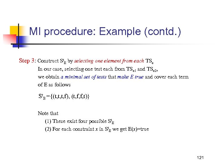
MI procedure: Example (contd. ) Step 3: Construct St. E by selecting one element from each TSe In our case, selecting one test each from TSe 1 and TSe 2, we obtain a minimal set of tests that make E true and cover each term of E as follows St. E ={(t, t, t, f), (t, f, f, t)} Note that (1) These exist four possible St. E (2) For each constraint x in St. E we get E(x)=true 121

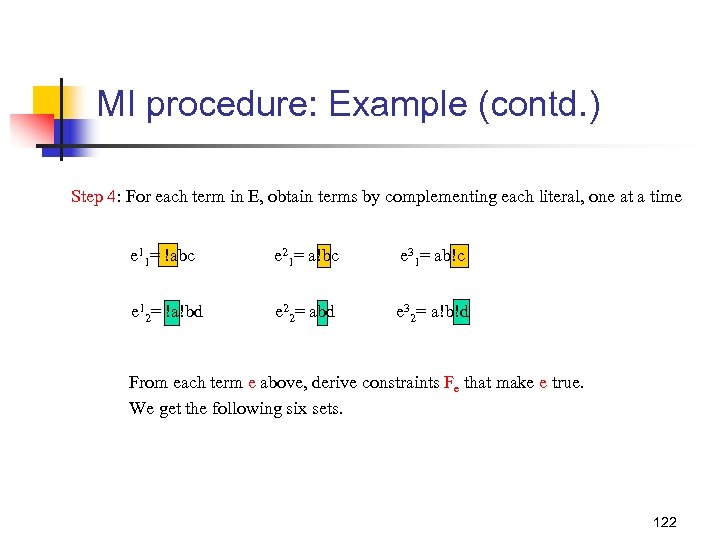
MI procedure: Example (contd. ) Step 4: For each term in E, obtain terms by complementing each literal, one at a time e 11= !abc e 21= a!bc e 31= ab!c e 12= !a!bd e 22= abd e 32= a!b!d From each term e above, derive constraints Fe that make e true. We get the following six sets. 122

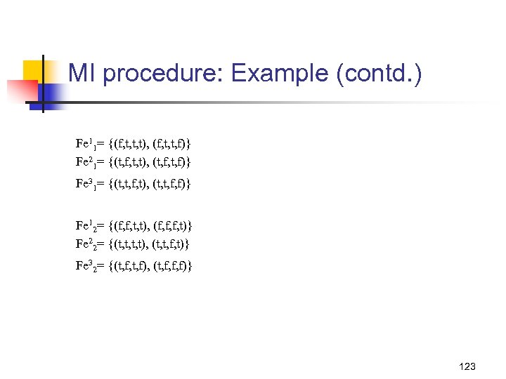
MI procedure: Example (contd. ) Fe 11= {(f, t, t, t), (f, t, t, f)} Fe 21= {(t, f, t, t), (t, f, t, f)} Fe 31= {(t, t, f, t), (t, t, f, f)} Fe 12= {(f, f, t, t), (f, f, f, t)} Fe 22= {(t, t, t, t), (t, t, f, t)} Fe 32= {(t, f, t, f), (t, f, f, f)} 123

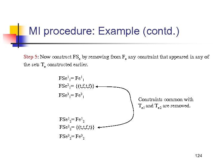
MI procedure: Example (contd. ) Step 5: Now construct FSe by removing from Fe any constraint that appeared in any of the sets Te constructed earlier. FSe 11= Fe 11 FSe 21= {(t, f, t, f)} FSe 31= Fe 31 Constraints common with Te 1 and Te 2 are removed. FSe 12= Fe 12 FSe 22= {(t, t, f, t)} FSe 32= Fe 32 124

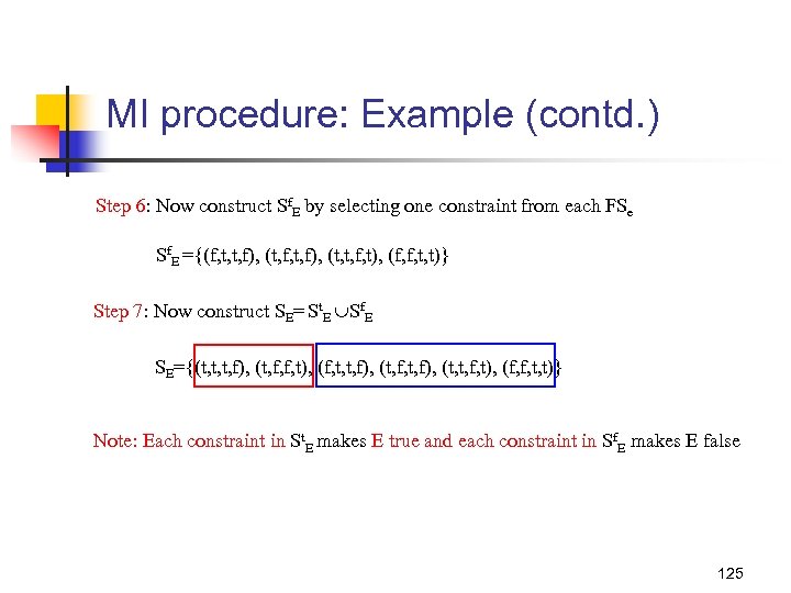
MI procedure: Example (contd. ) Step 6: Now construct Sf. E by selecting one constraint from each FSe Sf. E ={(f, t, t, f), (t, f, t, f), (t, t, f, t), (f, f, t, t)} Step 7: Now construct SE= St. E Sf. E SE={(t, t, t, f), (t, f, f, t), (f, t, t, f), (t, f, t, f), (t, t, f, t), (f, f, t, t)} Note: Each constraint in St. E makes E true and each constraint in Sf. E makes E false 125

BOR-MI-CSET procedure The BOR-MI-CSET procedure takes a possibly non-singular expression E as input and generates a constraint set that guarantees the detection of Boolean operator faults in the implementation of E The BOR-MI-CSET procedure using the MI procedure described earlier 126

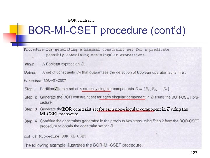
BOR constraint BOR-MI-CSET procedure (cont’d) E BOR constraint set for each non-singular component in E using the MI-CSET procedure 127

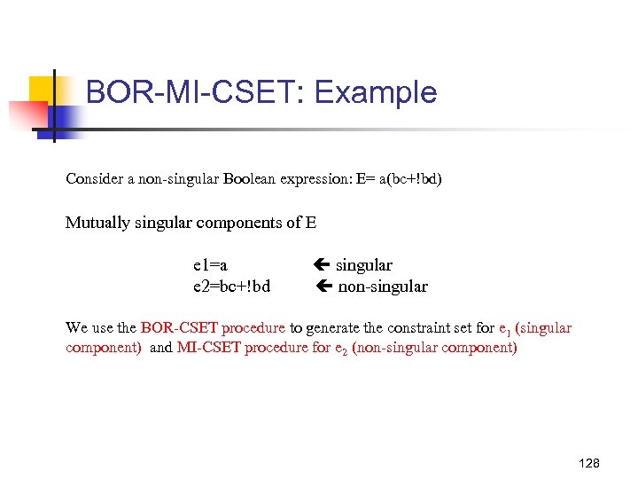
BOR-MI-CSET: Example Consider a non-singular Boolean expression: E= a(bc+!bd) Mutually singular components of E e 1=a e 2=bc+!bd singular non-singular We use the BOR-CSET procedure to generate the constraint set for e 1 (singular component) and MI-CSET procedure for e 2 (non-singular component) 128

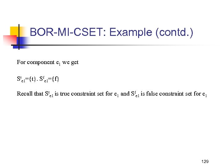
BOR-MI-CSET: Example (contd. ) For component e 1 we get Ste 1={t}. Sfe 1={f} Recall that Ste 1 is true constraint set for e 1 and Sfe 1 is false constraint set for e 1 129

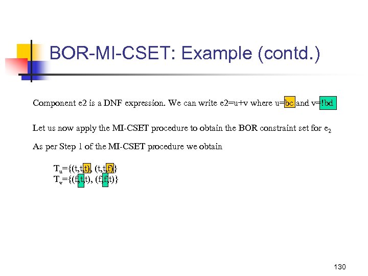
BOR-MI-CSET: Example (contd. ) Component e 2 is a DNF expression. We can write e 2=u+v where u=bc and v=!bd Let us now apply the MI-CSET procedure to obtain the BOR constraint set for e 2 As per Step 1 of the MI-CSET procedure we obtain Tu={(t, t, t), (t, t, f)} Tv={(f, t, t), (f, f, t)} 130

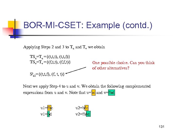
BOR-MI-CSET: Example (contd. ) Applying Steps 2 and 3 to Tu and Tv we obtain TSu=Tu ={(t, t, t), (t, t, f)} TSv=Tv ={(f, t, t), (f, f, t)} One possible choice. Can you think of other alternatives? Ste 2={(t, t, f), (f, t, t)} Next we apply Step 4 to u and v. We obtain the following complemented expressions from u and v. Note that u=bc and v=!bd u 1=!bc v 1=bd u 2=b!c v 2=!b!d 131

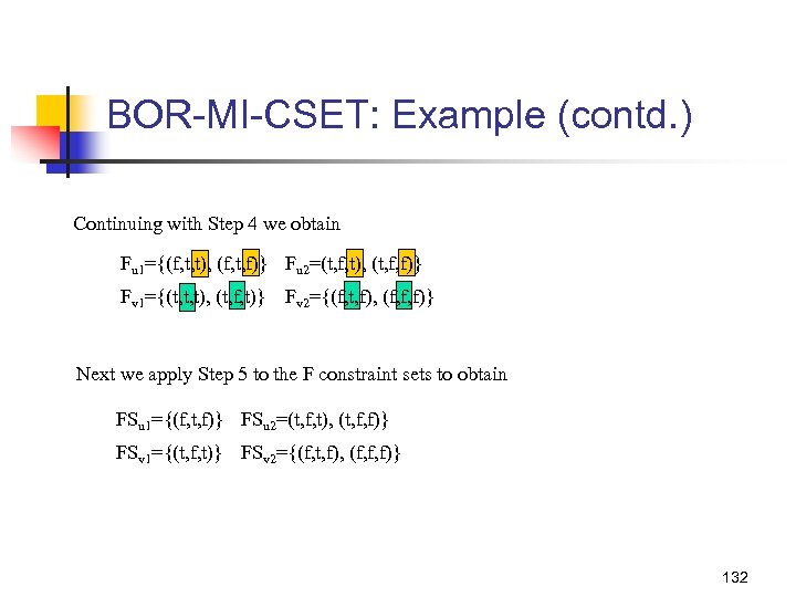
BOR-MI-CSET: Example (contd. ) Continuing with Step 4 we obtain Fu 1={(f, t, t), (f, t, f)} Fu 2=(t, f, t), (t, f, f)} Fv 1={(t, t, t), (t, f, t)} Fv 2={(f, t, f), (f, f, f)} Next we apply Step 5 to the F constraint sets to obtain FSu 1={(f, t, f)} FSu 2=(t, f, t), (t, f, f)} FSv 1={(t, f, t)} FSv 2={(f, t, f), (f, f, f)} 132

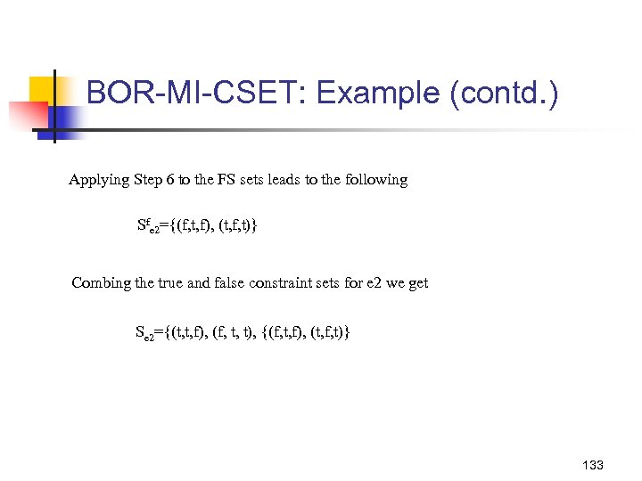
BOR-MI-CSET: Example (contd. ) Applying Step 6 to the FS sets leads to the following Sfe 2={(f, t, f), (t, f, t)} Combing the true and false constraint sets for e 2 we get Se 2={(t, t, f), (f, t, t), {(f, t, f), (t, f, t)} 133

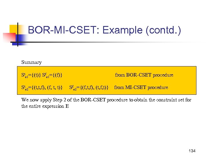
BOR-MI-CSET: Example (contd. ) Summary Ste 1={(t)} Sfe 1={(f)} Ste 2={(t, t, f), (f, t, t)} from BOR-CSET procedure Sfe 2={(f, t, f), (t, f, t)} from MI-CSET procedure We now apply Step 2 of the BOR-CSET procedure to obtain the constraint set for the entire expression E 134

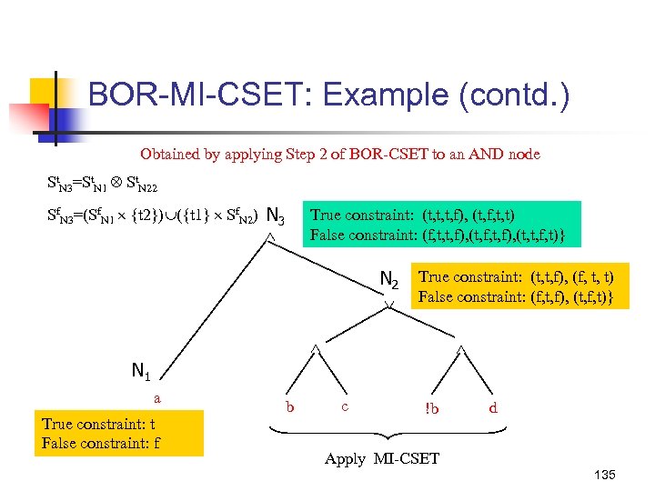
BOR-MI-CSET: Example (contd. ) Obtained by applying Step 2 of BOR-CSET to an AND node St. N 3=St. N 1 St. N 22 Sf. N 3=(Sf. N 1 {t 2}) ({t 1} Sf. N 2) N 3 True constraint: (t, t, t, f), (t, f, t, t) False constraint: (f, t, t, f), (t, f, t, f), (t, t, f, t)} N 2 True constraint: (t, t, f), (f, t, t) False constraint: (f, t, f), (t, f, t)} N 1 a True constraint: t False constraint: f b c !b d Apply MI-CSET 135

Summary Most requirements contain conditions under which functions are to be executed. Predicate testing procedures covered are excellent means to generate tests to ensure that each condition is tested adequately. 136

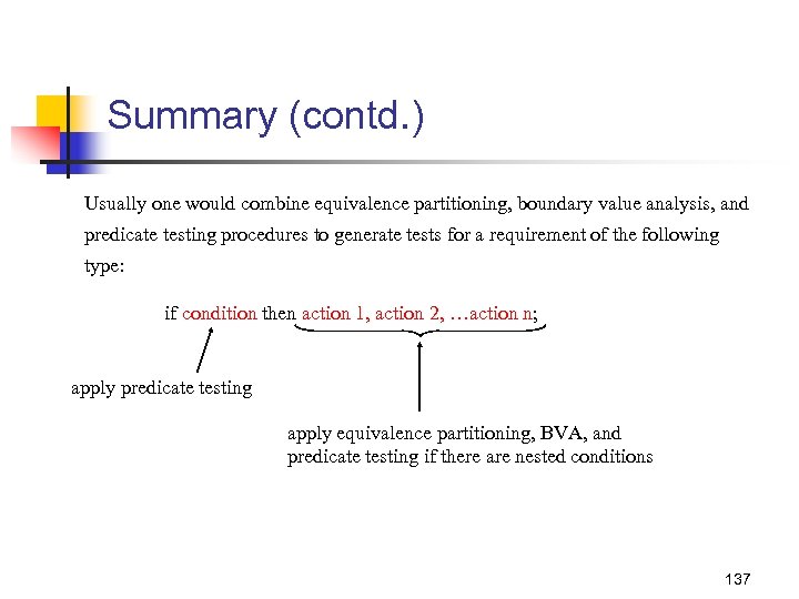
Summary (contd. ) Usually one would combine equivalence partitioning, boundary value analysis, and predicate testing procedures to generate tests for a requirement of the following type: if condition then action 1, action 2, …action n; apply predicate testing apply equivalence partitioning, BVA, and predicate testing if there are nested conditions 137