Regression Models Residuals and Diagnosing the Quality of

Regression Models Residuals and Diagnosing the Quality of a Model

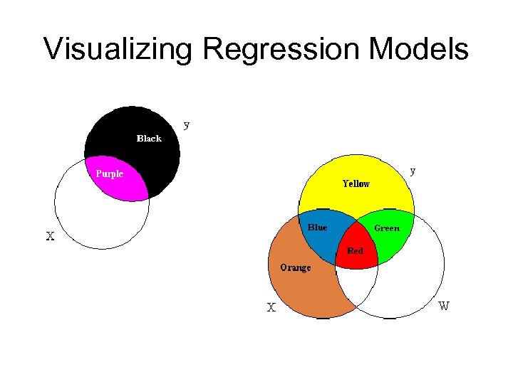
Visualizing Regression Models

Criteria of quality • Residuals (or what we don’t explain) should be “noise” • Independent variables measure different phenomena • We haven’t left out something important.

Diagnosing the Quality of a Regression Model Using the Residuals • Regression models assume that the errors of prediction are: – homoscedastic, – not autocorrelated, – normally distributed, and – not correlated with the independent variables.

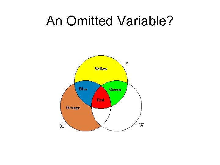
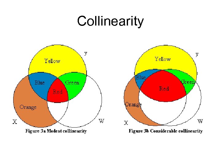
Regression Models assume… • The independent variables measure different phenomena, that is the independent variables are not themselves correlated. • If they are, we have a problem of “collinearity” or “multicolinearity. ”

Collinearity

An Omitted Variable?

Models • A Model: A statement of the relationship between a phenomenon to be explained and the factors, or variables, which explain it. • Steps in the Process of Quantitative Analysis: – Specification of the model – Estimation of the model – Evaluation of the model

Thus far… • We’ve discussed… – The specification of a model, – The estimation of a model and how to read and interpret the statistics we’ve produced: coefficients, t tests, F tests, R Square • Now we need to evaluate the model for problems and further elaboration.

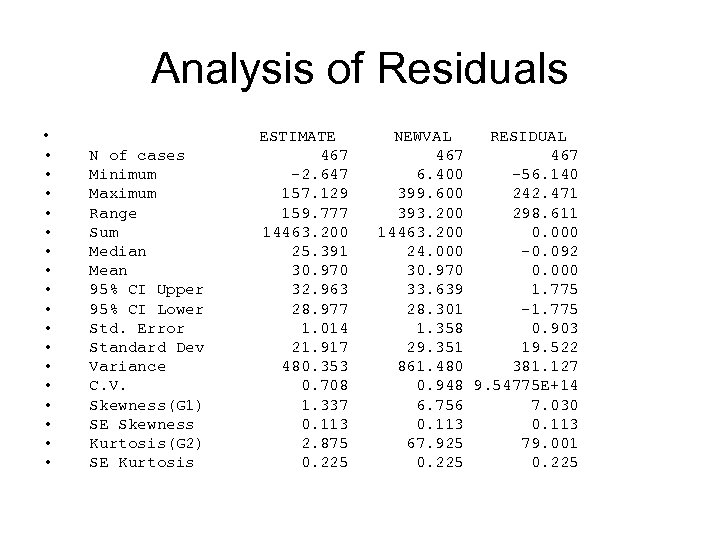
We need to evaluate • The variation in the predicted values and the difference between the Yi and the predicted Y. That difference is called a “residual. ” • We can analyze the residuals to see how good the equation is, and whethere are problems with the model that need correction or improvement.

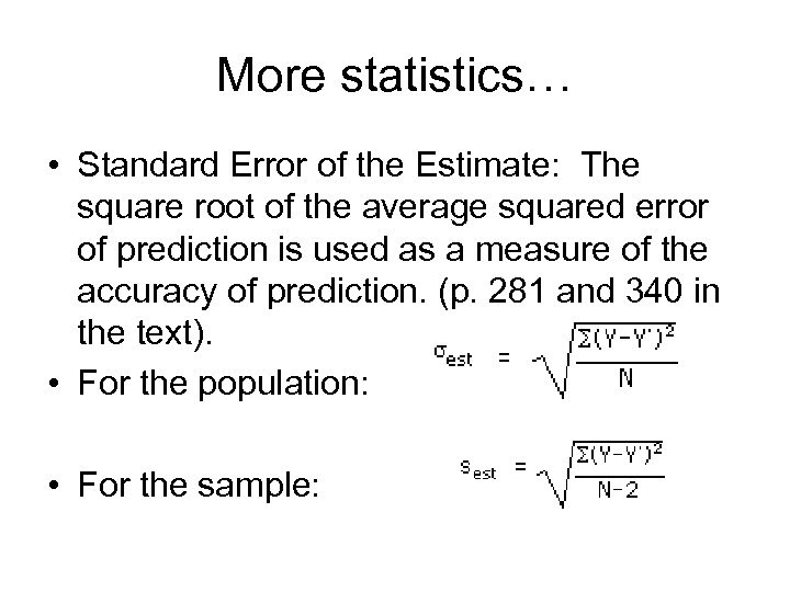More statistics… • Standard Error of the Estimate: The square root of the average squared error of prediction is used as a measure of the accuracy of prediction. (p. 281 and 340 in the text). • For the population: • For the sample:

Standard Error of the Estimate • Used to calculate a confidence interval around the predicted y. • As a rule of thumb, multiply the SEE by 2 and add and subtract from the predicted Ys to determine a measure of the variability of the prediction at a 95% confidence level. • At the mean of the independent variable: the standard error of the prediction = SEE/(square root of n).

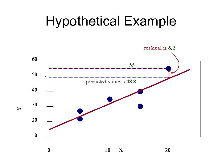
Hypothetical Example residual is 6. 2 60 55 50 predicted value is 48. 8 Y 40 30 20 10 X 20

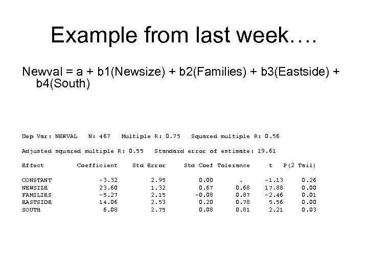Example from last week…. Newval = a + b 1(Newsize) + b 2(Families) + b 3(Eastside) + b 4(South) Dep Var: NEWVAL N: 467 Multiple R: 0. 75 Adjusted squared multiple R: 0. 55 Effect CONSTANT NEWSIZE FAMILIES EASTSIDE SOUTH Squared multiple R: 0. 56 Standard error of estimate: 19. 61 Coefficient Std Error -3. 32 23. 60 -5. 27 14. 06 6. 08 2. 95 1. 32 2. 15 2. 53 2. 75 Std Coef Tolerance 0. 00 0. 67 -0. 08 0. 20 0. 08 . 0. 68 0. 87 0. 78 0. 81 t -1. 13 17. 88 -2. 46 5. 56 2. 21 P(2 Tail) 0. 26 0. 00 0. 01 0. 00 0. 03

To understand the principles, let’s simplify…. • We return to the bivariate case: • House value is a function of the size of the building. • Regression models assume that the errors of prediction are homoscedastic, not autocorrelated, normally distributed, and not correlated with the independent variables. • That is, the error term should be noise. • Now we ask: – 1. how accurate our prediction is, – 2. what are the characteristics of the residuals or the error term.

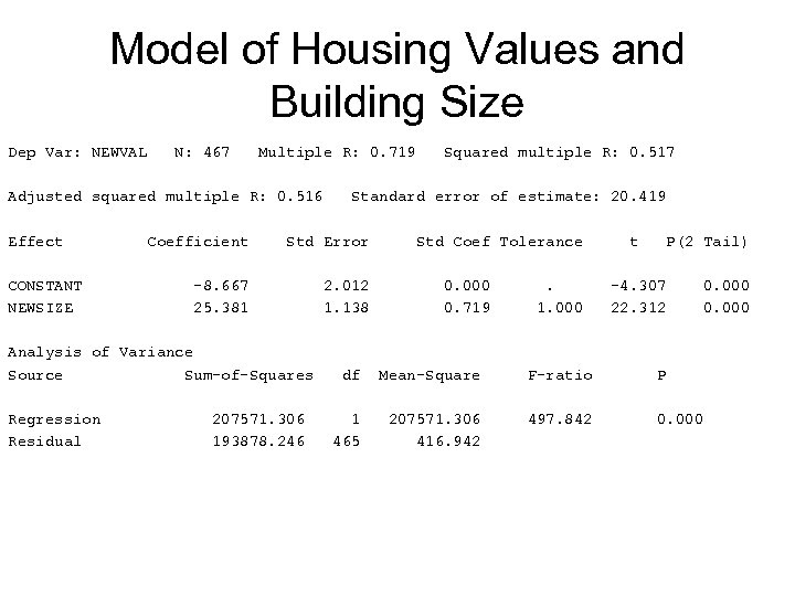Model of Housing Values and Building Size Dep Var: NEWVAL N: 467 Multiple R: 0. 719 Adjusted squared multiple R: 0. 516 Effect CONSTANT NEWSIZE Regression Residual Standard error of estimate: 20. 419 Coefficient Std Error -8. 667 25. 381 2. 012 1. 138 Analysis of Variance Source Sum-of-Squares 207571. 306 193878. 246 Squared multiple R: 0. 517 Std Coef Tolerance 0. 000 0. 719 . 1. 000 t P(2 Tail) -4. 307 22. 312 df Mean-Square F-ratio P 1 465 207571. 306 416. 942 497. 842 0. 000

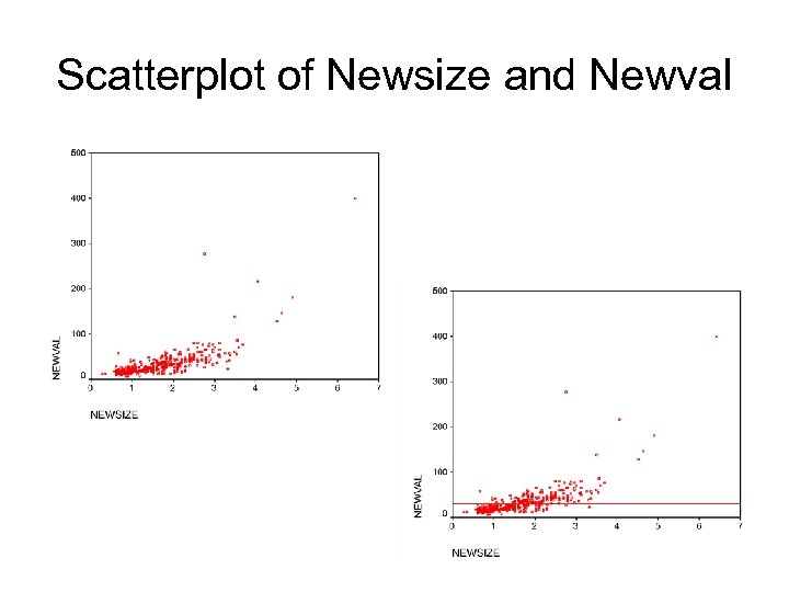Scatterplot of Newsize and Newval

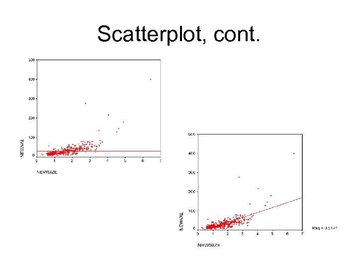Scatterplot, cont.

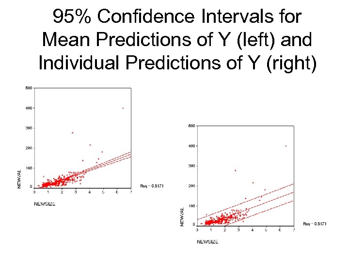95% Confidence Intervals for Mean Predictions of Y (left) and Individual Predictions of Y (right)

Hypothetical Example residual is 6. 2 60 55 50 predicted value is 48. 8 Y 40 30 20 10 X 20

Analysis of Residuals • • • • • N of cases Minimum Maximum Range Sum Median Mean 95% CI Upper 95% CI Lower Std. Error Standard Dev Variance C. V. Skewness(G 1) SE Skewness Kurtosis(G 2) SE Kurtosis ESTIMATE 467 -2. 647 157. 129 159. 777 14463. 200 25. 391 30. 970 32. 963 28. 977 1. 014 21. 917 480. 353 0. 708 1. 337 0. 113 2. 875 0. 225 NEWVAL RESIDUAL 467 6. 400 -56. 140 399. 600 242. 471 393. 200 298. 611 14463. 200 0. 000 24. 000 -0. 092 30. 970 0. 000 33. 639 1. 775 28. 301 -1. 775 1. 358 0. 903 29. 351 19. 522 861. 480 381. 127 0. 948 9. 54775 E+14 6. 756 7. 030 0. 113 67. 925 79. 001 0. 225

Visualizing Regression Models

Collinearity

An Omitted Variable?