REGRESSION MODEL WITH TWO EXPLANATORY VARIABLES MULTIPLE

REGRESSION MODEL WITH TWO EXPLANATORY VARIABLES

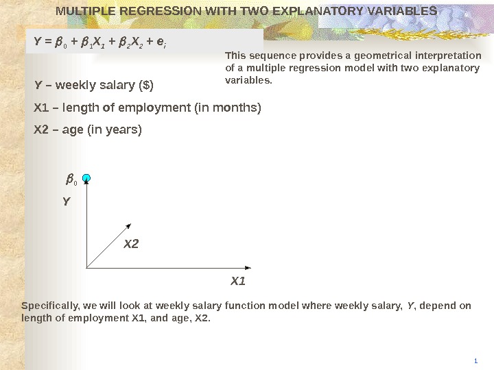
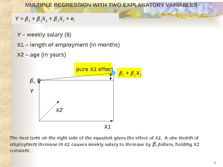
MULTIPLE REGRESSION WITH TWO EXPLANATORY VARIABLES Y X 2 X 10 Y = 0 + 1 X 1 + 2 X 2 + e i 1 This sequence provides a geometrical interpretation of a multiple regression model with two explanatory variables. Y – weekly salary ($) X 1 – length of employment (in months) X 2 – age (in years) Specifically, we will look at weekly salary function model where weekly salary, Y , depend on length of employment X 1, and age, X 2.

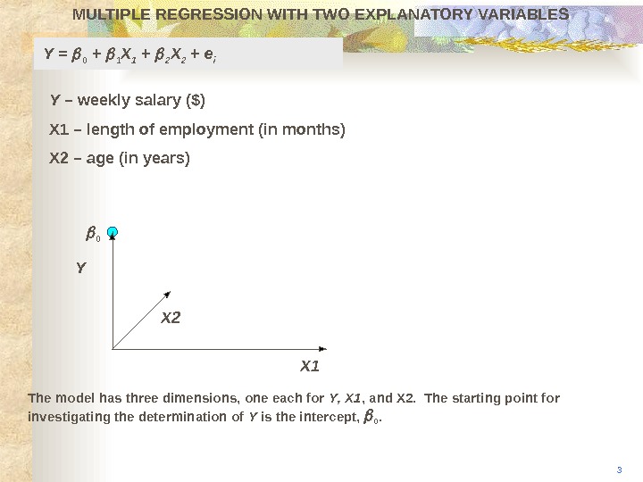
MULTIPLE REGRESSION WITH TWO EXPLANATORY VARIABLES Y X 2 X 10 3 The model has three dimensions, one each for Y , X 1 , and X 2. The starting point for investigating the determination of Y is the intercept, 0. Y = 0 + 1 X 1 + 2 X 2 + e i Y – weekly salary ($) X 1 – length of employment (in months) X 2 – age (in years)

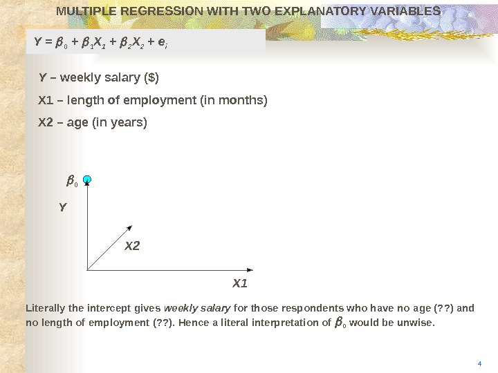
MULTIPLE REGRESSION WITH TWO EXPLANATORY VARIABLES Y X 2 X 10 4 Literally the intercept gives weekly salary for those respondents who have no age (? ? ) and no length of employment (? ? ). Hence a literal interpretation of 0 would be unwise. Y = 0 + 1 X 1 + 2 X 2 + e i Y – weekly salary ($) X 1 – length of employment (in months) X 2 – age (in years)

MULTIPLE REGRESSION WITH TWO EXPLANATORY VARIABLES 5 Y X 2 The next term on the right side of the equation gives the effect of X 1. A one month of employment increase in X 1 causes weekly salary to increase by 1 dollars, holding X 2 constant. X 1 0 pure X 1 effect 0 + 1 X 1 Y = 0 + 1 X 1 + 2 X 2 + e i Y – weekly salary ($) X 1 – length of employment (in months) X 2 – age (in years)

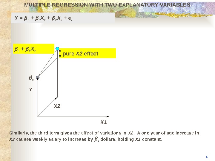
pure X 2 effect. MULTIPLE REGRESSION WITH TWO EXPLANATORY VARIABLES X 10 0 + 2 X 2 Y X 2 6 Similarly, the third term gives the effect of variations in X 2. A one year of age increase in X 2 causes weekly salary to increase by 2 dollars, holding X 1 constant. Y = 0 + 1 X 1 + 2 X 2 + e i

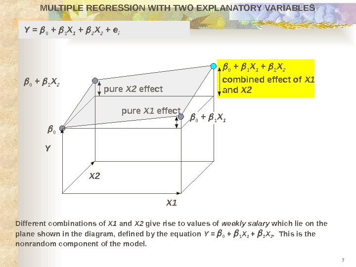
pure X 2 effect pure X 1 effect. MULTIPLE REGRESSION WITH TWO EXPLANATORY VARIABLES X 10 0 + 2 X 2 0 + 1 X 1 + 2 X 2 Y X 2 0 + 1 X 1 combined effect of X 1 and X 2 7 Different combinations of X 1 and X 2 give rise to values of weekly salary which lie on the plane shown in the diagram, defined by the equation Y = 0 + 1 X 1 + 2 X 2. This is the nonrandom component of the model. Y = 0 + 1 X 1 + 2 X 2 + e i

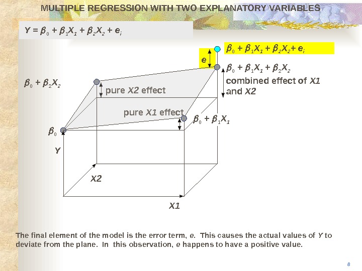
pure X 2 effect pure X 1 effect. MULTIPLE REGRESSION WITH TWO EXPLANATORY VARIABLES X 10 0 + 2 X 2 0 + 1 X 1 + 2 X 2 + e i Y X 2 combined effect of X 1 and X 2 e 8 The final element of the model is the error term, e. This causes the actual values of Y to deviate from the plane. In this observation, e happens to have a positive value. 0 + 1 X 1 Y = 0 + 1 X 1 + 2 X 2 + e i

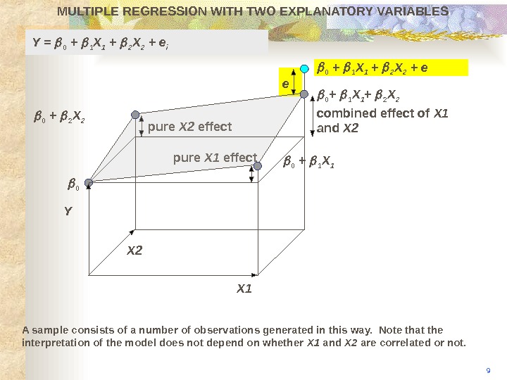
pure X 2 effect pure X 1 effect. MULTIPLE REGRESSION WITH TWO EXPLANATORY VARIABLES X 10 0 + 1 X 1 + 2 X 2 0 + 1 X 1 + 2 X 2 + e Y X 2 combined effect of X 1 and X 2 e 9 A sample consists of a number of observations generated in this way. Note that the interpretation of the model does not depend on whether X 1 and X 2 are correlated or not. 0 + 1 X 1 Y = 0 + 1 X 1 + 2 X 2 + e i 0 + 2 X

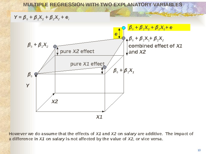
pure X 2 effect pure X 1 effect. MULTIPLE REGRESSION WITH TWO EXPLANATORY VARIABLES 10 X 10 0 + 1 X 1 + 2 X 2 + e Y X 2 combined effect of X 1 and X 2 e However we do assume that the effects of X 1 and X 2 on salary are additive. The impact of a difference in X 1 on salary is not affected by the value of X 2 , or vice versa. 0 + 1 X 1 Y = 0 + 1 X 1 + 2 X 2 + e i 0 + 2 X

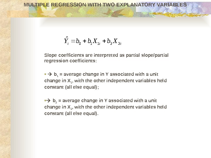
Slope coefficients are interpreted as partial slope/partial regression coefficients : b 1 = average change in Y associated with a unit change in X 1 , with the other independent variables held constant (all else equal) ; b 2 = average change in Y associated with a unit change in X 2 , with the other independent variables held constant (all else equal). MULTIPLE REGRESSION WITH TWO EXPLANATORY VARIABLESiii. Xbb. Y 22110 ˆ

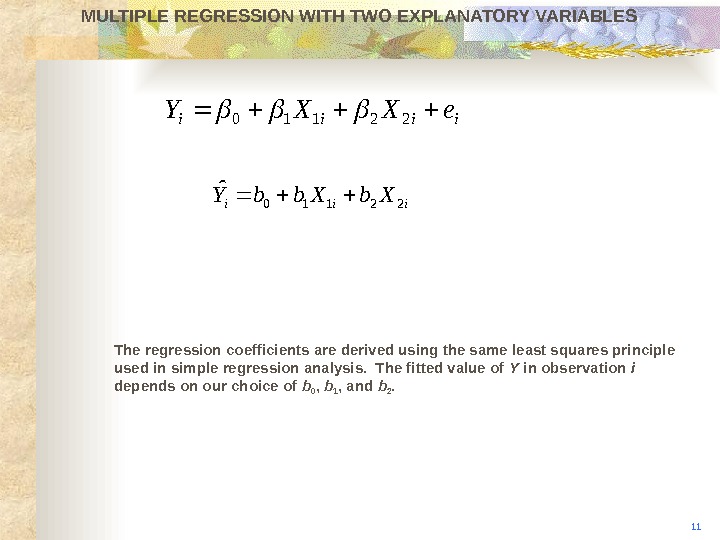
iiii e. XXY 22110 iii. Xbb. Y 22110 ˆMULTIPLE REGRESSION WITH TWO EXPLANATORY VARIABLES The regression coefficients are derived using the same least squares principle used in simple regression analysis. The fitted value of Y in observation i depends on our choice of b 0 , b 1 , and b 2.

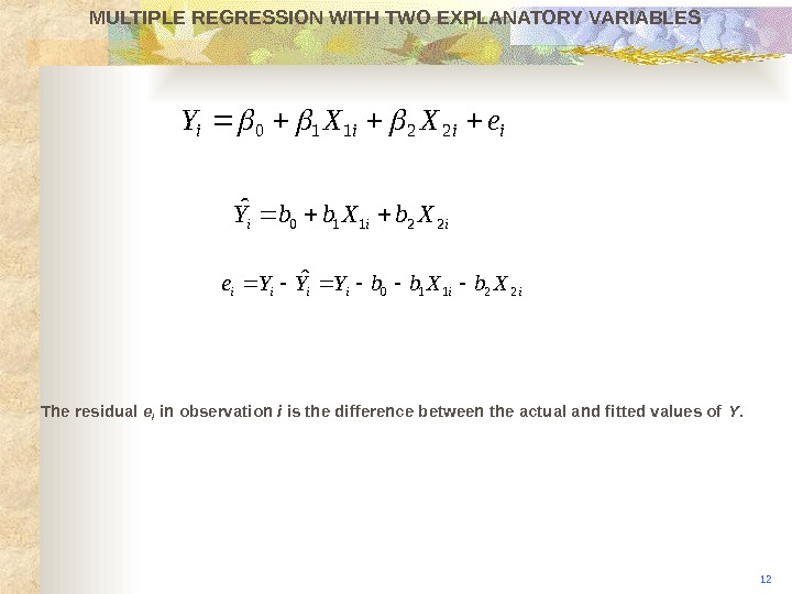
iiiiii. Xbb. YYYe 22110 ˆMULTIPLE REGRESSION WITH TWO EXPLANATORY VARIABLES The residual e i in observation i is the difference between the actual and fitted values of Y. 12 iiii e. XXY 22110 iii. Xbb. Y 22110 ˆ

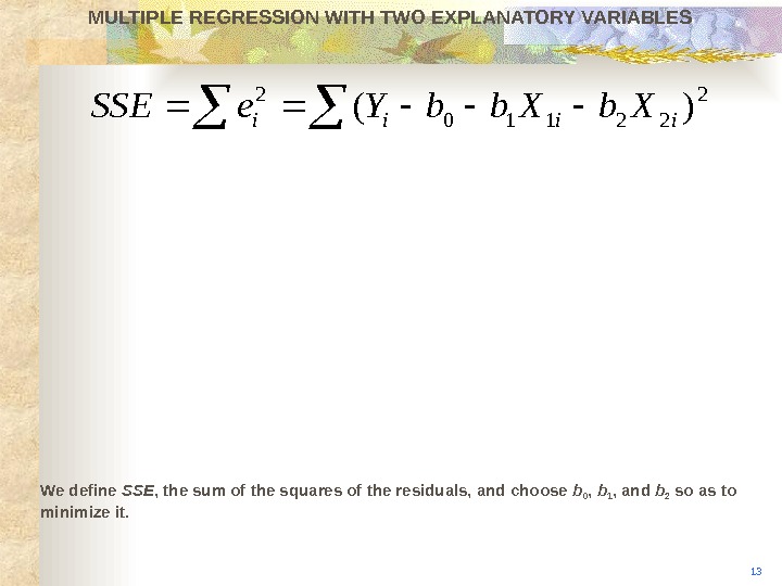
2 22110 2 )(iiii. Xbb. Ye. SSEMULTIPLE REGRESSION WITH TWO EXPLANATORY VARIABLES We define SS E , the sum of the squares of the residuals, and choose b 0 , b 1 , and b 2 so as to minimize it.

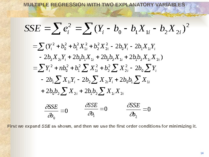
)2222 22( 212112011022 110 2 2 2 1 2 0 2 iiiiii XXbb. YXb. Yb. Xbb. Y iiiii XXbb. YXb Yb. Xbnb. Y 2121220 1102211 0 2 2 2 1 2 0 2 22 20 0 b. SSE 0 1 b. SSE 0 2 b. SSE MULTIPLE REGRESSION WITH TWO EXPLANATORY VARIABLES First we expand SS E as shown, and then we use the first order conditions for minimizing it. 14 2 22110 2 )(iiii. Xbb. Ye. SS

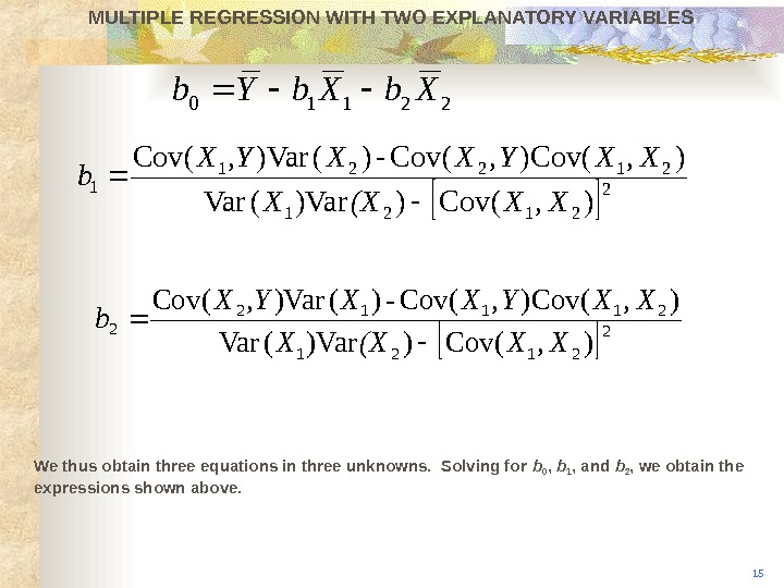
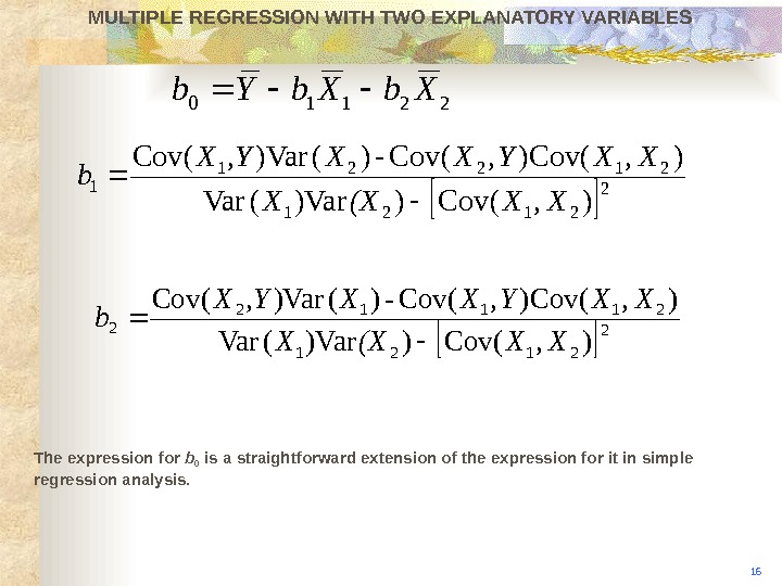
22110 Xb. Yb 2 2121 21221 1), (Cov))Var(Var ), (Cov-)()Var(Cov XX(XX XXYXX, YX b MULTIPLE REGRESSION WITH TWO EXPLANATORY VARIABLES We thus obtain three equations in three unknowns. Solving for b 0 , b 1 , and b 2 , we obtain the expressions shown above. 15 2 2121 21112 2 ), (Cov))Var(Var ), (Cov-)()Var(Cov XX(XX XXYXX, YX b

MULTIPLE REGRESSION WITH TWO EXPLANATORY VARIABLES The expression for b 0 is a straightforward extension of the expression for it in simple regression analysis. 1622110 Xb. Yb 2 2121 21221 1), (Cov))Var(Var ), (Cov-)()Var(Cov XX(XX XXYXX, YX b 2 2121 21112 2 ), (Cov))Var(Var ), (Cov-)()Var(Cov XX(XX XXYXX, YX b

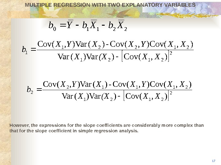
MULTIPLE REGRESSION WITH TWO EXPLANATORY VARIABLES However, the expressions for the slope coefficients are considerably more complex than that for the slope coefficient in simple regression analysis. 1722110 Xb. Yb 2 2121 21221 1), (Cov))Var(Var ), (Cov-)()Var(Cov XX(XX XXYXX, YX b 2 2121 21112 2 ), (Cov))Var(Var ), (Cov-)()Var(Cov XX(XX XXYXX, YX b

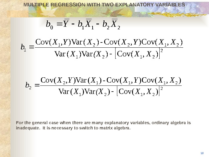
MULTIPLE REGRESSION WITH TWO EXPLANATORY VARIABLES For the general case when there are many explanatory variables, ordinary algebra is inadequate. It is necessary to switch to matrix algebra. 1822110 Xb. Yb 2 2121 21221 1), (Cov))Var(Var ), (Cov-)()Var(Cov XX(XX XXYXX, YX b 2 2121 21112 2 ), (Cov))Var(Var ), (Cov-)()Var(Cov XX(XX XXYXX, YX b

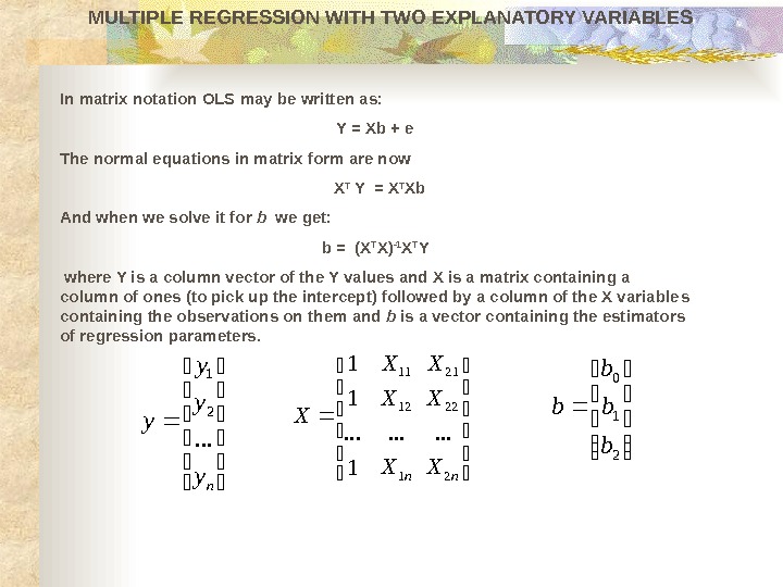
In matrix notation OLS may be written as: Y = Xb + e The normal equations in matrix form are now X T Y = X T Xb And when w e solve it for b we get: b = (X T X) -1 X T Y where Y is a column vector of the Y values and X is a matrix containing a column of ones (to pick up the intercept) followed by a column of the X variable s containing the observations on t hem and b is a vector containing the estimators of regression parameters. MULTIPLE REGRESSION WITH TWO EXPLANATORY VARIABLES ny y y y. . . 2 1 21 0 b b nn. X X X X 2 22 21 1 12 11. . .

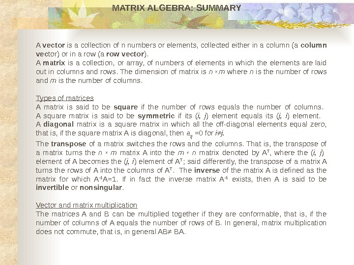
MATRIX ALGEBRA : SUMMARY A vector is a collection of n numbers or elements, collected either in a column (a column vec tor) or in a row (a row vector ). A matrix is a collection, or array, of numbers of elements in which the elements are laid out in columns and rows. The dimension of matrix is n x m where n is the number of rows and m is the number of columns. Types of matrices A matrix is said to be square if the number of rows equals the number of columns. A square matrix is said to be symmetric if its ( i, j ) element equals its ( j, i ) element. A diagonal matrix is a square matrix in which all the off-diagonal elements equal zero, that is, if the square matrix A is diagonal, then a ij =0 for i≠j. The transpose of a matrix switches the rows and the columns. That is, the transpose of a matrix turns the n x m matrix A into the m x n matrix denoted by A T , where the ( i, j ) element of A becomes the ( j, i ) element of A T ; said differently, the transpose of a matrix A turns the rows of A into the columns of A T. The inverse of the matrix A is defined as the matrix for which A -1 A= 1. If in fact the inverse matrix A -1 exists, then A is said to be invertible or nonsingular. Vector and matrix multiplication The matrices A and B can be multiplied together if they are conformable, that is, if the number of columns of A equals the number of rows of B. In general, matrix multiplication does not commute, that is, in general AB≠ BA.

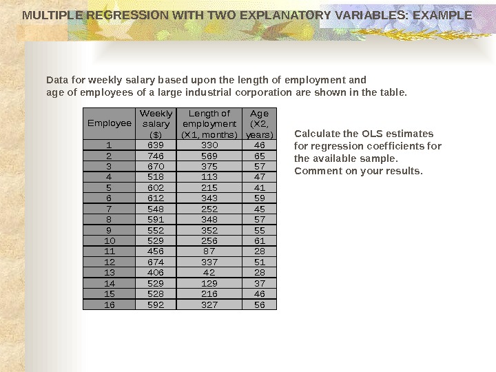
MULTIPLE REGRESSION WITH TWO EXPLANATORY VARIABLES: EXAMPLE Data for weekly salary based upon the length of employment and age of employees of a large industrial corporation are shown in the table. 163933046 274656965 367037557 451811347 560221541 661234359 754825245 859134857 955235255 1052925661 114568728 1267433751 134064228 1452912937 1552821646 1659232756 Weekly salary ($) Length of employment (X 1, months) Age (X 2, years) Employee Calculate the OLS estimates for regression coefficients for the available sample. Comment on your results.

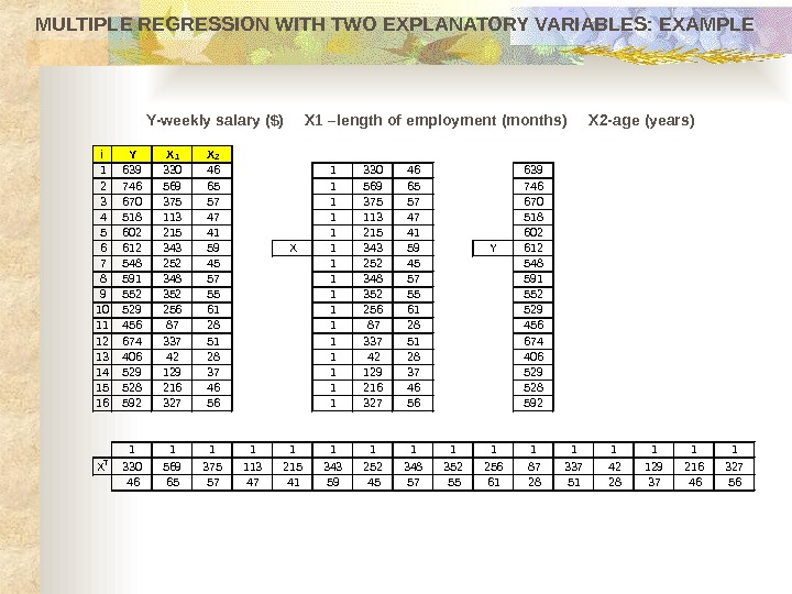
MULTIPLE REGRESSION WITH TWO EXPLANATORY VARIABLES: EXAMPLE i Y X 1 X 2 1 639 330 46 1 330 46 639 2 746 569 65 1 569 65 746 3 670 375 57 1 375 57 670 4 518 113 47 1 113 47 518 5 602 215 41 1 215 41 602 6 612 343 59 X 1 343 59 Y 612 7 548 252 45 1 252 45 548 8 591 348 57 591 9 552 352 55 1 352 55 552 10 529 256 61 1 256 61 529 11 456 87 28 1 87 28 456 12 674 337 51 1 337 51 674 13 406 42 28 1 42 28 406 14 529 129 37 1 129 37 529 15 528 216 46 1 216 46 528 16 592 327 56 1 327 56 592 1 1 1 1 X T 330 569 375 113 215 343 252 348 352 256 87 337 42 129 216 327 46 65 57 47 41 59 45 57 55 61 28 51 28 37 46 56 Y- weekly salary ($) X 1 – length of employment (month s) X 2 — age (years )

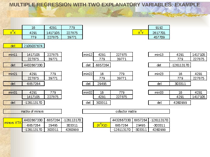
MULTIPLE REGRESSION WITH TWO EXPLANATORY VARIABLES: EXAMPLE 1642917799192 XTX 42911417105227875 XTY 2617701 77922787539771457709 det 2105037674 min 111417105227875 min 124291227875 min 1342911417105 22787539771779227875 det 4432667330 det-6857264 det -126113170 min 214291779 min 2216779 min 23164291 22787539771779227875 det-6857264 det 29495 det 303311 min 314291779 min 3216779 min 33164291 141710522787542911417105 det-126113170 det 303311 det 4260999 4432667330 -6857264 -12611317044326673306857264 -126113170 -685726429495303311(XTX)D 685726429495 -303311 -1261131703033114260999 -126113170 -3033114260999 minors XTX matrix of minorscofactor matrix

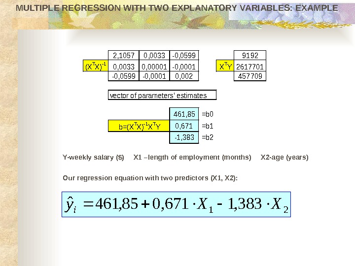
MULTIPLE REGRESSION WITH TWO EXPLANATORY VARIABLES: EXAMPLE 2, 10570, 0033 -0, 05999192 (XTX)-10, 00330, 00001 -0, 0001 XTY 2617701 -0, 0599 -0, 00010, 002457709 461, 85=b 0 0, 671=b 1 -1, 383=b 2 vector of parameters’ estimates b=(XTX)-1 XTY Y- weekly salary ($) X 1 – length of employment (month s) X 2 — age (years ) Our regression equation with two predictors (X 1, X 2): 21 383, 1671, 085, 461ˆ XXy i

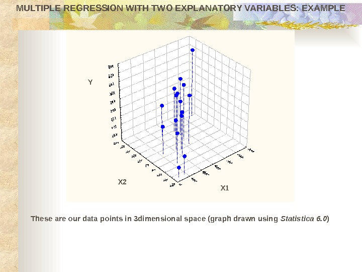
MULTIPLE REGRESSION WITH TWO EXPLANATORY VARIABLES: EXAMPLE These are our data points in 3 dimensional space (graph drawn using Statistica 6. 0 )X 1 X 1 Y X

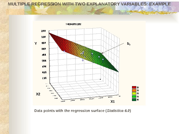
MULTIPLE REGRESSION WITH TWO EXPLANATORY VARIABLES: EXAMPLEY =461, 850+0, 671*X 1 -1, 383*X 2 800 700 600 500 400 Data points with the regression surface ( Statistica 6. 0 )X 1 X 2 Y b

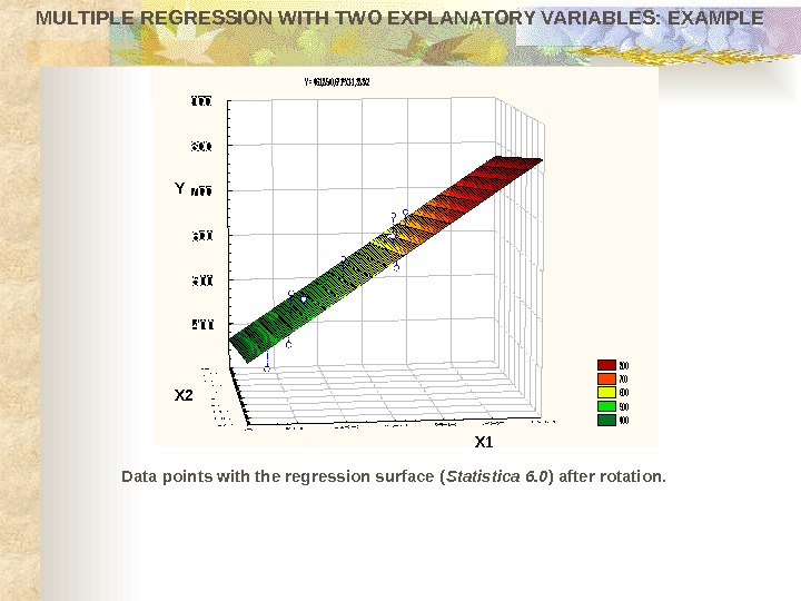
MULTIPLE REGRESSION WITH TWO EXPLANATORY VARIABLES: EXAMPLE Data points with the regression surface ( Statistica 6. 0 ) after rotation. Y = 461, 85+0, 671*X 1 -1, 383 X 2 800 700 600 500 400 Y X 1 X