Regression Analysis in Trials Peter T Donnan Professor

Regression Analysis in Trials Peter T. Donnan Professor of Epidemiology and Biostatistics

Objectives • Understand when to use regression modelling in trials • Regression for adjustment for baseline value of primary outcome • Regression for imbalance • Regression for subgroup analyses • Practical analysis using SPSS

Example data Pedometer trial CI Prof Mc. Murdo From trial of pedometers+advice vs controls in sedentary elderly women i. e. 3 arm trial Follow-up at 3 and 6 months Main outcome measure of activity from accelerometer counts at 3 months 210 randomised / 170 at 3 months

Type of Analyses – Pedometer trial 1. Compare mean final activity with ttests or ANOVA 2. Subtract baseline from final and compare CHANGE between groups with t-tests or ANOVA (sometimes as %) 3. Compare mean final activity with t-test adjusting for baseline activity (Regression or ANCOVA)

Type of Analyses – Pedometer trial Activity Advice only Pedometer Controls Difference in means at 3 months Baseline 3 -months 1. Compare mean final activity with t-tests or ANOVA

Type of Analyses – Pedometer trial Activity Advice only Pedometer Controls CHANGE between baseline and 3 months Baseline 2. 3 -months Subtract baseline from final and compare CHANGE between groups with t-tests or ANOVA

Problems with CHANGE or % CHANGE Regression to the mean – extreme values at baseline will tend to drift towards mean e. g. very low baseline values correlated with high change even if no effect of intervention If low correlation between baseline measure and follow-up then using CHANGE will add variation and follow-up more likely to show significance Regression approach more efficient (unless correlation > 0. 8)

Best approach to analysing ‘Change’ Fit model with baseline measure as covariate and indicator variable for arm of trial (A vs. B) Follow-up score = constant + a x baseline score + b x arm Where b represents the difference between the two arms of the trial i. e. the intervention ‘effect’ adjusted for the baseline value and so represents ‘change’

Pedometer trial Regression Analyses Best analysis is regression model (or ANCOVA) Linear regression as outcome continuous Primary Outcome 3 mnth activity – Accel. VM 2 Want to compare Pedom Vs. control (GRP 1) and Advice vs. control (GRp 2) – so create 2 dummy variables Important adjustment variable is the baseline Accel. VM 1 a

Example data – Pedometer trial Read in data ‘SPSS Study databse. sav’ Main outcome is: 3 mnth activity – Accel. VM 2 Baseline activity – Accel. VM 1 a Trial arm represented by two dummy variables: Grp 1 = Pedom. Vs. control Grp 2 = Advice vs. control

Example data – Pedometer trial Carry out the three ways of analysing the outcome 1. Final 3 months activity only (Accel. VM 2) 2. Change between 3 months activity and baseline (Diff. VM_3 mn) 3. Regression on 3 months activity (Accel. VM 2) adjusting for baseline activity (Accel. VM 1 a)

Pedometer trial – 1) Analysis of 3 months only Descriptives Accel. VM 2 N Pedometer Group 58 Advice only 52 Controls 62 Total 172 Mean 145383. 79 138343. 81 123843. 65 135490. 95 SD 52585. 7 54708. 9 51090. 5 53201. 6 95% CI for Mean 131557. 08 159210. 50 123112. 74 153574. 87 110869. 10 136818. 19 127483. 52 143498. 39 No significant difference but Pedometer arm highest activity (p = 0. 076 ANOVA)

Pedometer trial – 2) Analysis of CHANGE 3 months (difference 3 months and baseline) Diffvm_3 mn N Mean Std. Deviation Pedometer Group 58 5504. 3 34010. 2 Advice only 52 13305. 3 37084. 9 Controls 61 -2290. 3 29020. 9 Total 171 5096. 0 33733. 1 Significant difference but Advice CHANGE greatest (p = 0. 042 ANOVA)

Pedometer trial -Analysis of CHANGE 3 months + Run-in After run-in period Pedometer group started highest and so Advice group started lowest and rose most!

Pedometer trial –Notes on analysis of PERCENTAGE CHANGE 3 months Analysis by %CHANGE similar problems to analysis of CHANGE but…. . also creates non-normality and does NOT allow for imbalance at baseline (Vickers, 2001) Still o. k. to calculate results as % change for presentation purposes but analysis is more efficient as adjusted regression

Pedometer trial – 3) regression analysis adjusting for baseline 3) Regression on 3 months activity adjusting for baseline activity and two dummy variables representing trial arm contrasts

Main analysis – Pedometer trial N. b. Pedom vs Control p=0. 117 Advice vs Control p = 0. 014 Baseline Accel. VM 1 a highly sig.

Differences in baseline characteristics Characteristics Age in years, mean (SD) Marital status, n (%) Married Widowed Single Used pedometer before, n (%) No Yes Illness, n (%) No Yes Daily stairs, n (%) No Yes Stairs difficult, n (%) No Yes All (n = 210) 77. 28 (5. 04) 91 (43. 3) 96 (45. 7) 23 (10. 9) 196 (93. 3) 14 (6. 7) 146 (69. 5) 64 (30. 5) 84 (40. 0) 126 (60. 0) 143 (68. 1) 67 (31. 9) Randomised Group (6 missing) 1 (n = 68) 2 (n = 68) 3 (n = 68) 77. 15 (4. 89) 77. 56 (5. 43) 76. 96 (4. 93) 26 (38. 2) 34 (50. 0) 29 (42. 6) 36 (52. 9) 22 (32. 4) 33 (48. 5) 6 (8. 8) 12 (17. 6) 5 (7. 4) 63 (92. 6) 64 (94. 1) 63 (92. 6) 5 (7. 4) 4 (5. 9) 5 (7. 4) 45 (66. 2) 43 (63. 2) 53 (77. 9) 23 (33. 8) 25 (36. 8) 15 (22. 1) 23 (33. 8) 28 (41. 2) 30 (44. 1) 45 (66. 2) 40 (58. 8) 30 (55. 9) 48 (70. 6) 45 (66. 2) 20 (29. 4) 23 (33. 8)

Differences in baseline characteristics Characteristics All (n = 210) Randomised Group (6 missing) 1 (n = 68) 2 (n = 68) 3 (n = 68) Season entered, n (%) Winter 82 (39. 0) 29 (42. 6) 26 (38. 2) Spring 69 (32. 9) 20 (29. 4) 24 (35. 3) 23 (33. 8) Summer 40 (19. 0) 14 (20. 6) 11 (16. 2) 13 (19. 1) Autumn 19 (9. 0) 5 (7. 4) 7 (10. 3) 6 (8. 8) Lives with, n (%) 113 (53. 8) 39 (57. 4) 31 (45. 6) 38 (55. 9) 2 (1. 0) 29 (42. 6) 37 (54. 4) 30 (44. 1) 0 172 (81. 9) 58 (85. 3) 52 (76. 5) 62 (91. 2) 1 7 (3. 3) 0 (0. 0) 4 (5. 9) 3 (4. 4) 2+ 8 (3. 9) 4 (5. 9) 3 (4. 4) 1 (1. 5) Alone With someone Falls in last 3 months, n (%) 1 st 3 months of study

Imbalance in baseline characteristics • Despite randomisation there are some characteristics that are not BALANCED across the three arms of the trial • More likely to get imbalance in smaller trials • One solution is to adjust for these imbalances in regression of final outcome • Alternatives are to use STRATIFICATION, or MINIMISATION when allocating eligible subjects to treatment in design • n. b. do NOT test for differences across arms as not primary hypothesis!

Imbalance in baseline characteristics • Repeat the regression analysis but adding baseline characteristics as covariates in the regression model • What variables should you adjust for? • These need to be stated in SAP prior to data analysis

Pedometer trial Regression Analyses Regression Coefficients Factors Final regression model adjusting for a number of baseline factors Intercept Beta Std. Error t p-value 0. 540 0. 590 26613. 5 49272. 8 Pedometer Group vs. controls 10064. 5 6030. 6 1. 669 0. 097 Advice only vs. controls 18056. 5 6242. 3 2. 893 0. 004 All active vs. controls 13799. 8 5270. 2 2. 618 0. 010 Age -678. 3 577. 5 -1. 175 0. 242 Limb total at baseline 2070. 0 1277. 2 1. 621 0. 107 Stairs difficult 13081. 2 6017. 1 2. 174 0. 031 Total no. of drugs -1325. 9 794. 1 -1. 670 0. 097 6471. 7 5323. 2 1. 216 0. 226 13. 11 8. 52 1. 539 0. 126 Living Alone Health Costs at baseline

Summary Pedometer Trial • Regression adjustment most appropriate method for analysing change • Significant - advice only vs. Controls • Pedometer - approaching significance • Perhaps run-in should be counted as part of intervention but protocol stipulated comparison of change between baseline and 3 months ignoring the run-in • Be careful how analysis is framed in protocol!

Pedometer Trial paper Mc. Murdo MET, Sugden J, Argo I, Boyle P, Johnston DW, Sniehotta FF, Donnan PT. Do pedometers increase physical activity in sedentary older women? A randomised controlled trial. J Am Geriatr Soc, 2010; 58(11): 2099 -106.

Example outcome with categorical - Bell’s Palsy Trial Background Ø A multicentre factorial trial of the early administration of steroids and/or antivirals for Bell’s palsy What is Bell’s Palsy? BP is an acute unilateral paralysis of the facial nerve Its cause is unknown; it affects between 25 to 30 people per 100, 000 population per annum; most common within 30 and 45 years old higher prevalence in: pregnant women, diabetes, influenza, upper respiratory ailment

What the patient notices I couldn’t whistle. (Graeme Garden et al) Things tasted odd: my Mac. Donald’s tasted awful. (BELLS pt, Edinburgh) My food fell out of my mouth. (BELLS pt, Dundee) I winked at my husband. He jumped. (BELLS pt, Montrose)

Background and Aim 2003: in UK 36% were treated with steroids; 19% were referred to Hospital and 45% were untreated Most recover well but up to 30% had poor recovery: Facial disfigurement Psychological difficulties Facial pain To conduct a cost-effectiveness and costutility analyses alongside the clinical RCT

RCT Design A randomised 2 x 2 factorial design To assess: prednisolone (steroids) and/or acyclovir (antiviral) commenced within 72 hours of onset of BP result in the same level of disability and pain after 9 months as treatment with placebo. Patient randomised received 2 identical preparations for 10 days simultaneously: Prednisolone (50 mg per day) + placebo Acyclovir (2000 mg per day) + placebo Prednisolone + Acyclovir Placebo + placebo

Inclusion Criteria and Outcomes Inclusion criteria: Adults (>16), no identifiable cause unilateral facial nerve weakness seen within 72 hours of onset Outcome measures: 1. House-Brackman grading system 2. Health Utility Index Mark III 3. Chronic pain grade 4. Costs (PC, Lo. S, outpatient visits, medications)

Measurement of Primary Outcomes at 3 months and 9 months I However, if patient “cured”, this is, H-B grading of 1, the individual was no longer followed-up II Then, IV subjects not cured at 3 months data on baseline, 3 months and 9 months post randomisation subjects cured at 3 months only have data at baseline and 3 months III V VI Normal symmetrical function in all areas Slight weakness Slight asymmetry of smile Obvious weakness, but not disfiguring Obvious disfiguring weakness Motion barely perceptible Incomplete eye closure, slight movement corner mouth No movement, loss of tone

Posed portrait photographs at onset eyebrows raised eyes tightly closed smiling

Posed portrait photographs at 3 months eyebrows raised eyes tightly closed smiling

Results follow Randomisation – No significant interactions Prednisolone x Aciclovir interaction at 3 months p = 0. 32 Prednisolone x Aciclovir interaction at 9 months p = 0. 72 Two trials for the price of one!

Results follow Randomisation Aciclovir No Aciclovir Adjusted OR (95% CI)* H-B I 3 months 71. 2% 75. 7% 0. 86 (0. 55, 1. 34) H-B I 9 months 85. 4% 90. 8% 0. 61 (0. 33, 1. 11) * Adjusted for age, sex, baseline H-B, interval from onset.

Results follow Randomisation Prednisolone No Adjusted OR Prednisolone (95% CI)* H-B I 3 months 83. 0% 63. 6% 2. 44 (1. 55, 3. 84) H-B I 9 months 94. 4% 81. 6% 3. 32 (1. 72, 6. 44) * Adjusted for age, sex, baseline H-B, interval from onset.

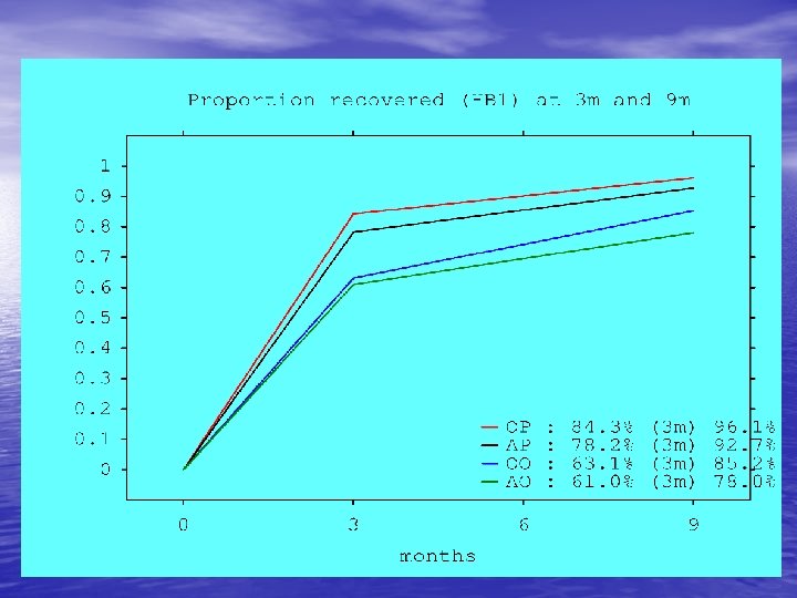
Summary Bell’s • Recovery at 9 months – 78% Acyclovir – 85% Placebo – 96% Prednisolone recover • NNT 6 at 3 months • NNT 8 at 9 months • The basis for sensible discussion of treatment options with patients • The type of study which is difficult to do without a primary care research network

Bell’s Palsy Trial paper Sullivan FM, Swan RC, Donnan PT, Morrison JM, Smith BH, Mc. Kinstry B, Vale L, Davenport RJ, Clarkson JE, Daly F. Early treatment with prednisolone or acyclovir and recovery in Bell’s palsy. NEJM 2007; 357: 1598 -607

Subgroup analysis

Incorrect approach to subgroup analysis • No mention of subgroup analysis in protocol • After testing initial primary hypothesis, test separately if results differ by: • Males vs females, Age groups, • Baseline severity, • Deprivation status, • High / low BP, • Etc……. . ad infinitum! • Bound to find something significant by chance alone (Type I error) and then report!

Correct approach to subgroup analysis • Must be pre-specified in the protocol and SAP prior to data lock • Test if results differ by subgroup by fitting the appropriate interaction term in a regression model • E. g. Treatment arm (0, 1) x Gender (0, 1) • If statistically significant then present results separately by group but strength of evidence needs interpretation.

Issues with subgroup analysis • Interpretation of subgroup analyses still contentious even if statistically correct • Subgroup analyses will be underpowered • Subgroup analyses tend to be overinterpretated by trialists (Pocock et al 2002) • Biological plausibility needs to be considered • Number should be limited due to problem of multiple testing

Summary • Three examples of use of regression modelling in RCTs • 1) Adjustment for baseline imbalances using logistic regression – Bell’s Palsy • 2) adjustment for baseline measure of primary outcome with multiple linear regression -Pedometer Trial

Summary • 3) Adding interaction terms to test for subgroup differences in treatment effect • Regression analysis type could be linear (continuous outcome), logistic (binary outcome, Cox (survival outcome) or counts (Poisson) • All easily fitted in SPSS or other statistical software

References • Analysing controlled trials with baseline and follow-up measurements. Vickers AJ, Altman DG. BMJ 2001; 323: 11234 • The use of percentage change from baseline as an outcome in a controlled trial is statistically inefficient: a simulation study. Vickers A. BMC Medical Research Methodology 2001; 1: 6. • Subgroup analysis, covariate adjustment and baseline comparisons in clinical trial reporting: current practice and problems. Pocock SJ, Assmann SE, Enos LE, Kasten LE. Statist Med 2002; 21: 2917 -2930.