b8152c018403aa0da6c5671b6de2ed18.ppt
- Количество слайдов: 62
Reducing Selection Bias via Propensity Score Approach Bo Lu, Ph. D. Division of Biostatistics College of Public Health The Ohio State University U. S. A KNAW, March 29, 2007 1
Outline n n n Overview: causal inference Real example: evaluation of training program Theory on propensity score Simulation example Implementation of propensity score matching Revisit the real example KNAW, March 29, 2007 2
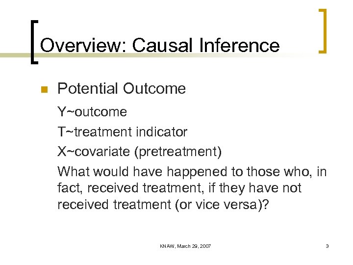
Overview: Causal Inference n Potential Outcome Y~outcome T~treatment indicator X~covariate (pretreatment) What would have happened to those who, in fact, received treatment, if they have not received treatment (or vice versa)? KNAW, March 29, 2007 3
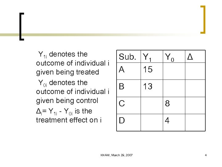
Y 1 i denotes the outcome of individual i given being treated Y 0 i denotes the outcome of individual i given being control Δi= Y 1 i - Y 0 i is the treatment effect on i Sub. Y 1 A 15 B Y 0 Δ 13 C 8 D 4 KNAW, March 29, 2007 4
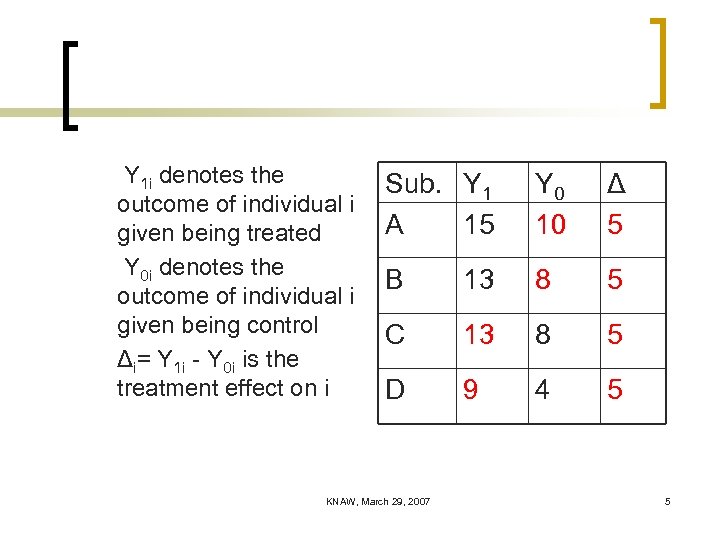
Y 1 i denotes the outcome of individual i given being treated Y 0 i denotes the outcome of individual i given being control Δi= Y 1 i - Y 0 i is the treatment effect on i Sub. Y 1 A 15 Y 0 10 Δ 5 B 13 8 5 C 13 8 5 D 9 4 5 KNAW, March 29, 2007 5
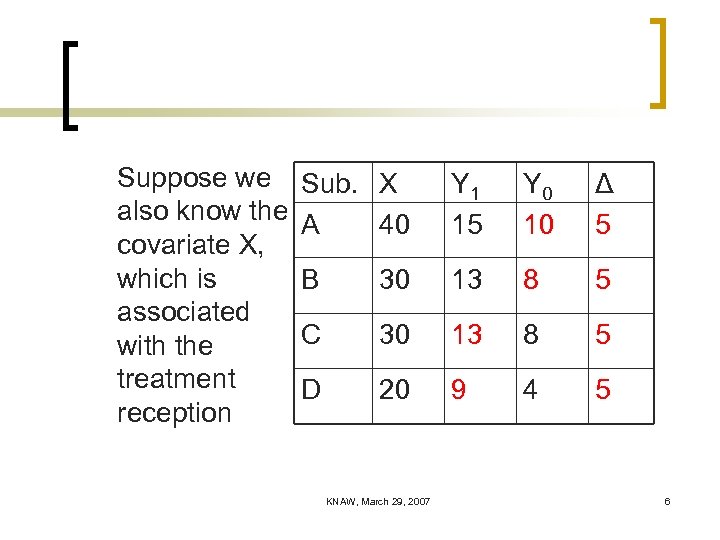
Suppose we also know the covariate X, which is associated with the treatment reception Sub. X A 40 Y 1 15 Y 0 10 Δ 5 B 30 13 8 5 C 30 13 8 5 D 20 9 4 5 KNAW, March 29, 2007 6
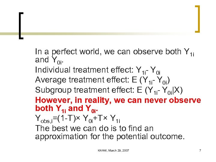
In a perfect world, we can observe both Y 1 i and Y 0 i. Individual treatment effect: Y 1 i- Y 0 i Average treatment effect: E (Y 1 i- Y 0 i) Subgroup treatment effect: E (Y 1 i- Y 0 i|X) However, in reality, we can never observe both Y 1 i and Y 0 i. Yobs, i=(1 -T)× Y 0 i+T× Y 1 i The best we can do is to find an approximation for the potential outcome. KNAW, March 29, 2007 7
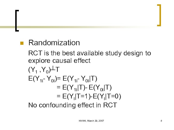
n Randomization RCT is the best available study design to explore causal effect (Y 1 , Y 0)┴T E(Y 1 i- Y 0 i)= E(Y 1 i- Y 0 i|T) = E(Y 1 i|T)- E(Y 0 i|T) = E(Yi|T=1)-E(Yi|T=0) No confounding effect in RCT KNAW, March 29, 2007 8
RCT has its own limitations: - RCT is not feasible for all causal effect studies—unethical, legal issues, etc - Small RCT may still suffer from unbalanced covariate distribution - Large RCT could be both costly and timeconsuming KNAW, March 29, 2007 9
- The units in observational studies are usually more representative, since randomized studies generally have to be conducted in a restricted environment. - Many studies designed as randomized experiments become more like observational studies when protocols are broken KNAW, March 29, 2007 10
n Observational Studies - treatment assignment is not random - the study could be carried out in a timeand money-efficient manner - traditional statistical analysis may provide biased results due to the self-selection into treatment KNAW, March 29, 2007 11
Example: Evaluation of Training Program n National Supported Work (NSW) Demonstration A randomized study implemented in the mid 1970 s to provide work experience for a period of 6 -18 months to individual who had faced economic and social problems. Outcome: difference in annual earning between pre- and post-intervention KNAW, March 29, 2007 12
n Lalonde’s Analysis (1986) - Estimate from experimental data - Estimate from non-experimental data: combine treated subjects in NSW with control subjects from PSID or CPS - Pre-intervention characteristics: age, education, Black, Hispanic, nodegree, married, earnings in 74 and 75 KNAW, March 29, 2007 13
- linear regression, fixed-effects and latent variable selection model n Dehejia and Wahba’s analysis (1999) - re-analyze the data with propensity score matching/stratification KNAW, March 29, 2007 14
Theory on Propensity Scores n n First established in the seminal paper by Rosenbaum and Rubin (1983) Assumptions - Stable unit treatment value assumption (SUTVA) The response of subject i to the treatment T does not depend on the treatment given to subject j. KNAW, March 29, 2007 15
- Strongly ignorable treatment assignment assumption (Y 1 , Y 0)┴T|X, conditional independence 0<P(T=1|X)<1, common support e(x)=P(T=1|x) is defined as the propensity score, which is a scalar summary of all observed covariates KNAW, March 29, 2007 16
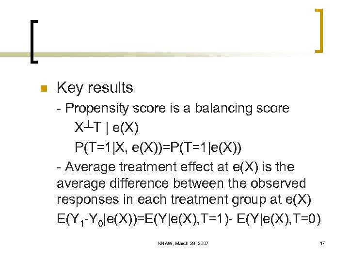
n Key results - Propensity score is a balancing score X┴T | e(X) P(T=1|X, e(X))=P(T=1|e(X)) - Average treatment effect at e(X) is the average difference between the observed responses in each treatment group at e(X) E(Y 1 -Y 0|e(X))=E(Y|e(X), T=1)- E(Y|e(X), T=0) KNAW, March 29, 2007 17
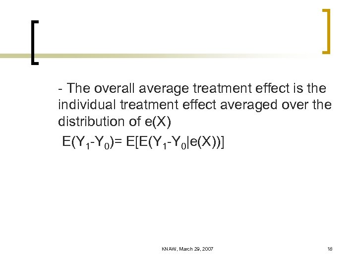
- The overall average treatment effect is the individual treatment effect averaged over the distribution of e(X) E(Y 1 -Y 0)= E[E(Y 1 -Y 0|e(X))] KNAW, March 29, 2007 18
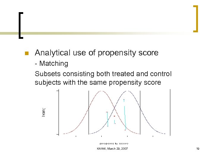
n Analytical use of propensity score - Matching Subsets consisting both treated and control subjects with the same propensity score KNAW, March 29, 2007 19
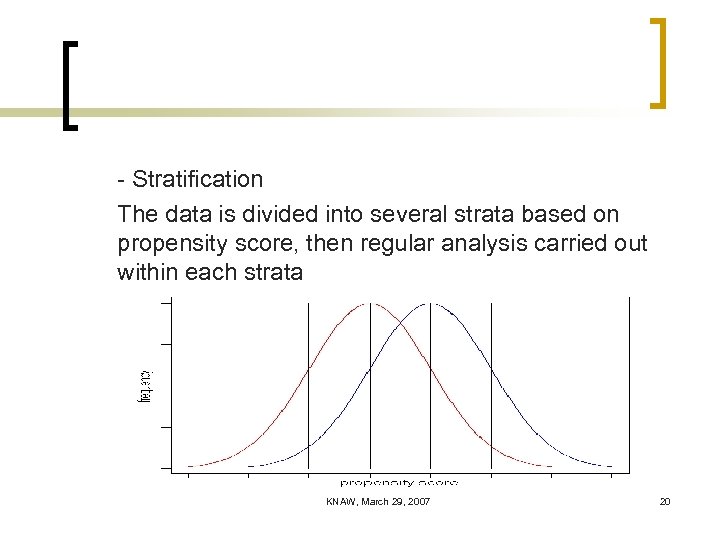
- Stratification The data is divided into several strata based on propensity score, then regular analysis carried out within each strata KNAW, March 29, 2007 20
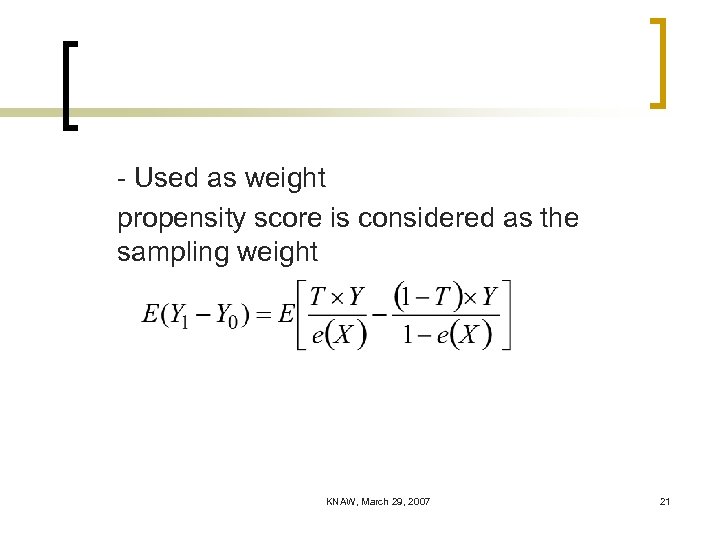
- Used as weight propensity score is considered as the sampling weight KNAW, March 29, 2007 21
Simulation Example n Simulation Setup T: treatment indicator (1, 0) X: covariate, normally distributed T=1, N(16, 4), n 1=200 T=0, N(10, 25), n 0=1000 Y: outcome, determined by hypothetical models KNAW, March 29, 2007 22
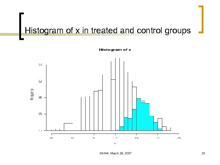
Histogram of x in treated and control groups KNAW, March 29, 2007 23
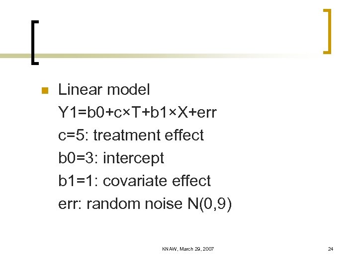
n Linear model Y 1=b 0+c×T+b 1×X+err c=5: treatment effect b 0=3: intercept b 1=1: covariate effect err: random noise N(0, 9) KNAW, March 29, 2007 24
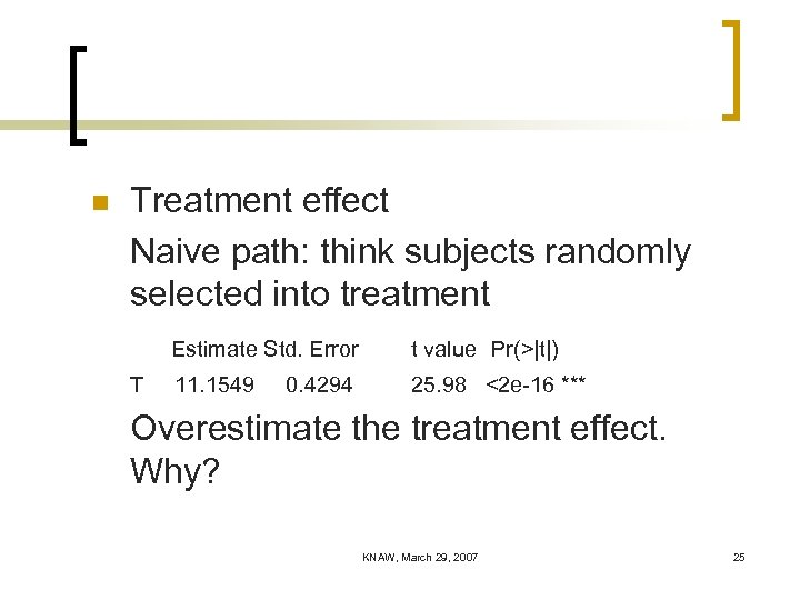
n Treatment effect Naive path: think subjects randomly selected into treatment Estimate Std. Error T t value Pr(>|t|) 11. 1549 25. 98 <2 e-16 *** 0. 4294 Overestimate the treatment effect. Why? KNAW, March 29, 2007 25
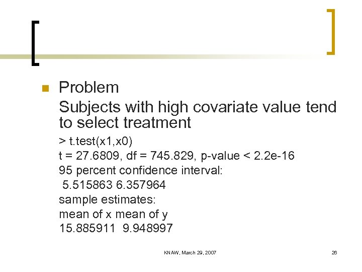
n Problem Subjects with high covariate value tend to select treatment > t. test(x 1, x 0) t = 27. 6809, df = 745. 829, p-value < 2. 2 e-16 95 percent confidence interval: 5. 515863 6. 357964 sample estimates: mean of x mean of y 15. 885911 9. 948997 KNAW, March 29, 2007 26
n Matching to balance the covariate distribution To make the treated and control subject look alike before treatment To produce a study regime which resembles a randomized experiment most, in terms of the observed covariates KNAW, March 29, 2007 27
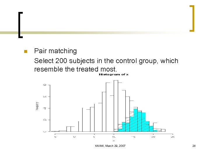
n Pair matching Select 200 subjects in the control group, which resemble the treated most. KNAW, March 29, 2007 28
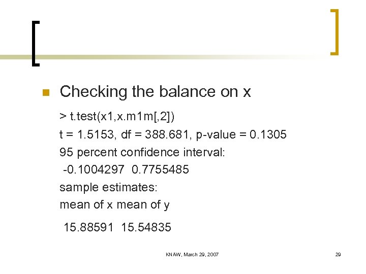
n Checking the balance on x > t. test(x 1, x. m 1 m[, 2]) t = 1. 5153, df = 388. 681, p-value = 0. 1305 95 percent confidence interval: -0. 1004297 0. 7755485 sample estimates: mean of x mean of y 15. 88591 15. 54835 KNAW, March 29, 2007 29
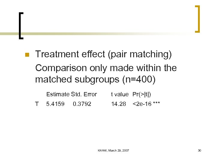
n Treatment effect (pair matching) Comparison only made within the matched subgroups (n=400) Estimate Std. Error T t value Pr(>|t|) 5. 4159 14. 28 0. 3792 KNAW, March 29, 2007 <2 e-16 *** 30
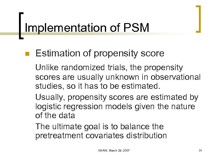
Implementation of PSM n Estimation of propensity score Unlike randomized trials, the propensity scores are usually unknown in observational studies, so it has to be estimated. Usually, propensity scores are estimated by logistic regression models given the nature of the data The ultimate goal is to balance the pretreatment covariates distribution KNAW, March 29, 2007 31
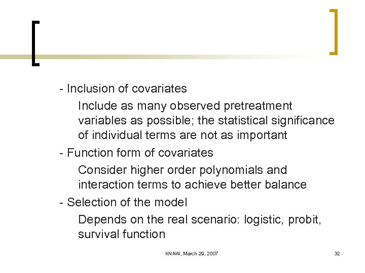
- Inclusion of covariates Include as many observed pretreatment variables as possible; the statistical significance of individual terms are not as important - Function form of covariates Consider higher order polynomials and interaction terms to achieve better balance - Selection of the model Depends on the real scenario: logistic, probit, survival function KNAW, March 29, 2007 32
n Matching algorithms - Nearest Neighbor algorithm Iteratively find the pair of subjects with the shortest distance Easy to understand implement; Offers good results in practice; fast running time; Rarely offers the best matching results (compared to optimal matching) KNAW, March 29, 2007 33
- Optimal algorithm To minimize the total distance for the overall population Offers the “best” matching results overall; Runs reasonably fast; Implementation is not easy; Not readily to extend to n-cube matching (n>2) KNAW, March 29, 2007 34
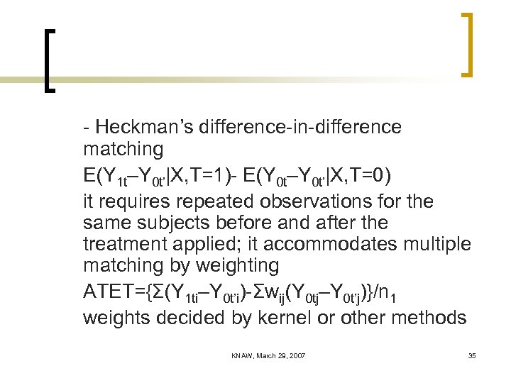
- Heckman’s difference-in-difference matching E(Y 1 t–Y 0 t’|X, T=1)- E(Y 0 t–Y 0 t’|X, T=0) it requires repeated observations for the same subjects before and after the treatment applied; it accommodates multiple matching by weighting ATET={Σ(Y 1 ti–Y 0 t’i)-Σwij(Y 0 tj–Y 0 t’j)}/n 1 weights decided by kernel or other methods KNAW, March 29, 2007 35
- Choices of distance exact match not possible, use one distance measure to summarize the information * Mahalanobis distance * Propensity score * Mahalanobis distance with propensity score caliper * Any distance with the requirement of exact match on a specific variable KNAW, March 29, 2007 36
n Matching Design - Bi-partite matching Pair matching: used when the numbers of the treated and control are comparable 1 -K matching: used when control group is huge compared to the treated Variable matching: more flexible than 1 -K, the matched control is set to be between a and b for each treated subject KNAW, March 29, 2007 37
Full matching: a way of sub-classification generalizing variable matching; each matched group contains one treated and multiple control or one control with multiple treated KNAW, March 29, 2007 38
- Non-bipartite Matching When there are multiple treatment groups or one treatment group with several control groups or treatment status changing over time Pair matching 1 -K matching Require special algorithm (complicated!) KNAW, March 29, 2007 39
n Available Software - SAS procs by Bergstralh, Kosanke, Jacobsen (1996) “Software for Optimal Matching in Observational Studies”, Epidemiology, 7, 331 -332 http: //mayoresearch. mayo. edu/mayo/research/biost at/sasmacros. cfm Bipartite matching: pair, 1 -k, variable KNAW, March 29, 2007 40
- R functions by Ben Hansen http: //www. stat. lsa. umich. edu/~bbh/# full matching - STATA function by Abadie, et al. http: //elsa. berkeley. edu/~imbens/statamatching. pdf Nearest Neighbor matching, estimating treatment effect proposed in econ literatures: SATE, PATE, SATT, etc KNAW, March 29, 2007 41
- STATA functions by Leuven & Sianesi psmatch 2() http: //athena. sas. upenn. edu/~petra/copen/statadoc. pdf Mahalanobis or propensity score distance matching for various designs : pair, kernel, local linear and spline matching (based on nearest-neighbor matching) KNAW, March 29, 2007 42
- R functions for optimal matching (under development) Core algorithms: a. FORTRAN codes for optimal nonbipartite matching by Derigs (1988) b. C codes for optimal weighted matching http: //elib. zib. de/pub/Packages/mathprog/matching/ weighted/ KNAW, March 29, 2007 43

Loaded into R with. Fortran()/. C() No Fortran or C compiler needed Downloadable on line Works under both UNIX and WINDOWS - UNIX: load. so file - WINDOWS: load. dll file Further questions, contact Bo Lu blu@cph. osu. edu KNAW, March 29, 2007 44
n Practical issues - Matching vs. Covariance adjustment modeling Matching: always reduce the bias; no worry about the true regression equation; easy post-matching analysis; restricted to common support Covariance adjustment modeling: has to guess the true regression equation (prone to bias); apply to the full range of the data; may lead to smaller variance estimation KNAW, March 29, 2007 45
- Exact matching vs. Complete matching Exact: balanced treated and control group; less usable data (treated cases may be excluded) Complete: try to use all data; less balanced covariate distribution; may need postmatching regression adjustment KNAW, March 29, 2007 46
n Procedure for PSM - Identify propensity score model - Estimate the propensity score with all data - Compute the distance between any two subjects - Create matched pair/group using a specific matching algorithm KNAW, March 29, 2007 47
- Check covariate balance between the treated and control among the matched subjects; If not good enough, go back to improve propensity score model - Contrast between the treated and control subjects within each pair/group - Obtain the average treatment effect by averaging over all pairs/groups KNAW, March 29, 2007 48
Revisit The Example The goal is to investigate the credibility of the conventional analytical results from nonexperimental data So, the authors compared the results from the experimental data and the results from non-experimental data by combining the treated with an existing comparable control dataset. KNAW, March 29, 2007 49
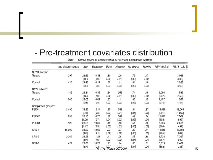
- Pre-treatment covariates distribution KNAW, March 29, 2007 50
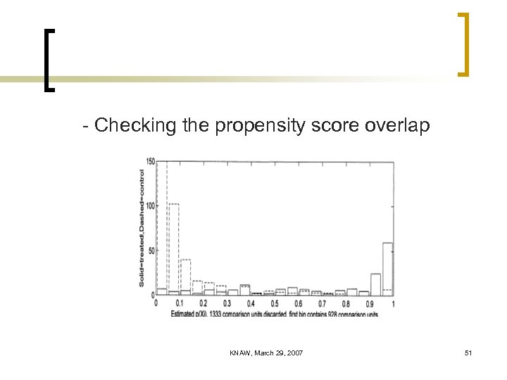
- Checking the propensity score overlap KNAW, March 29, 2007 51
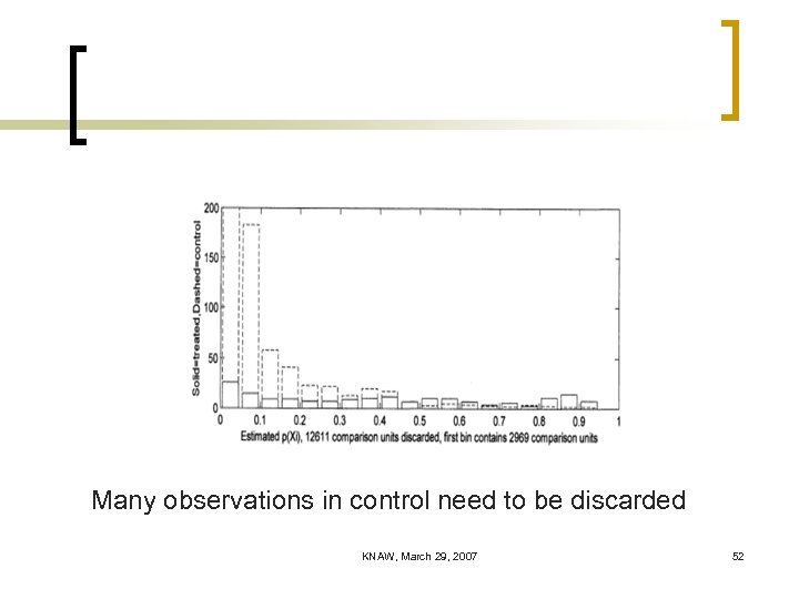
Many observations in control need to be discarded KNAW, March 29, 2007 52
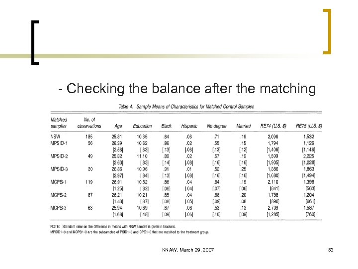
- Checking the balance after the matching KNAW, March 29, 2007 53
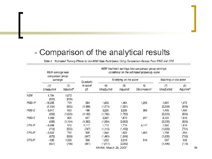
- Comparison of the analytical results KNAW, March 29, 2007 54
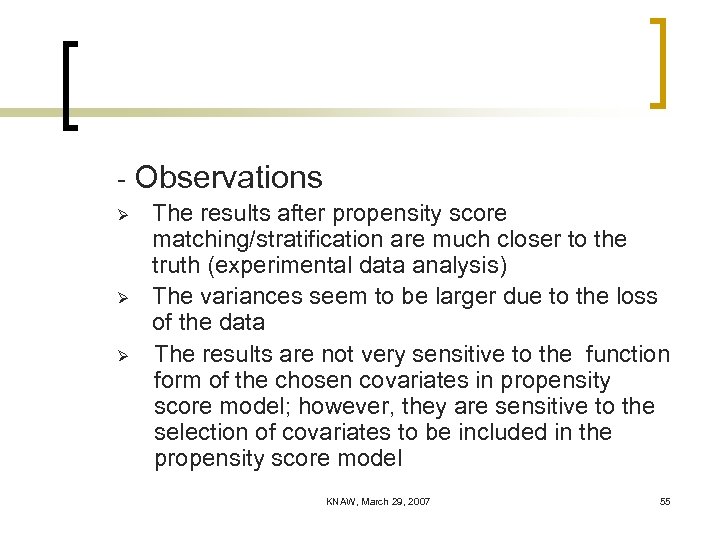
- Observations Ø Ø Ø The results after propensity score matching/stratification are much closer to the truth (experimental data analysis) The variances seem to be larger due to the loss of the data The results are not very sensitive to the function form of the chosen covariates in propensity score model; however, they are sensitive to the selection of covariates to be included in the propensity score model KNAW, March 29, 2007 55
Limitations and new advances n Limitation of PS method - Rely on a unverifiable assumption: strongly ignorable treatment assignment given the observed covariates Unlike the randomized studies, it has no control over the unobserved confounders One possible solution is to use sensitivity analysis to evaluate to what degree the results will change given a hypothesized unknown covariate KNAW, March 29, 2007 56
- Need substantial overlap between the treated and the control groups, otherwise, it may result in significant loss of the data in analysis One possible solution is to use regressionlike technique to extrapolate; however, such extrapolation might not be reliable KNAW, March 29, 2007 57
n Apply propensity score in longitudinal studies construct time-dependent propensity score - sequential matching - inverse-probability-of treatment weighted (IPTW) estimator KNAW, March 29, 2007 58
Reference n n n D’Agostino (1998), “Propensity score methods for bias reduction in the comparison of a treatment to a nonrandomized control group”, Stat. Med. 17, 2265 -2281. Dehejie & Wahba (1999), “Causal effects in nonexperimental studies: Reevaluating the evaluation of training programs”, JASA, 94, 1053 -1062. Dergis (1988), “Solving non-bipartite matching problem via shortest path techniques”, Annals of Operations Research, 13, 225 -261. Joffe & Rosenbaum (1999), “Propensity scores”, American J. of Epi. , 150, 327 -333. Imbens (2004), “Nonparametric estimation of average treatment effects under exogeneity”, Review of economics and statistics, 86, 4 -29. KNAW, March 29, 2007 59
n n n Lalonde (1986), “Evaluating the econometric evaluations of training programs”, American Economic Review, 76, 604 -620. Lu (2005), “Propensity score matching with time dependent covariates”, Biometrics, 61, 721 -728. Lu, Zanutto, Hornik & Rosenbaum (2001), “Matching with doses in an observational study of a media campaign against drug abuse”. Robins, Hernan & Brumback (2000), “Marginal structural models and causal inference in epidemiology”, Epidemiology, 11, 550 -560. Rosenbaum (1987), “Model-based direct adjustment”, JASA, 82, 387 -394. KNAW, March 29, 2007 60
n n n Rosenbaum (1989), “Optimal matching for observational studies”, JASA, 84, 1024 -1032. Rosenbaum (2002), Observatioal Studies, 2 nd Edition, Springer. Rosenbaum & Rubin (1983), “The central role of the propensity score in observational studies for causal effect”, Biometrika, 70, 41 -55. Rosenbaum & Rubin (1985), “The bias due to incomplete matching”, Biometrics, 41, 103 -116. Rubin (2005), “Causal inference using potential outcomes: Design, Modeling, Decision”, JASA, 100, 322 -331. KNAW, March 29, 2007 61
Acknowledgement My research on optimal nonbipartite matching was partially supported by funding provided by a seed grant from OSU's Initiative in Population Research Center Grant (NICHD, R 21, HD-47943 -03) KNAW, March 29, 2007 62
b8152c018403aa0da6c5671b6de2ed18.ppt