Real-Time Systems Real-time research repository For

Real-Time Systems

Real-time research repository § For information on real-time research groups, conferences, journals, books, products, etc. , have a look at: http: //cs-www. bu. edu/pub/ieee-rts/Home. html

Introduction § A real-time system is a system whose specification includes both a logical and a temporal correctness requirement. § Logical correctness: produce correct output. § Can be checked by various means including Hoare axiomatics and other formal methods. § Temporal correctness: produces output at the right time. § A soft real-time system is one that can tolerate some delay in delivering the result. § A hard real-time system is one that can not afford to miss a dealine.

Characteristics of real-time systems § § § Event-driven, reactive High cost of failure Concurrency/multiprogramming Stand-alone/continuous operation. Reliability/fault tolerance requirements PREDICTABLE BEHAVIOR

Misconceptions about real-time systems § There is no science in real-time-system design. § We shall see… § Advances in supercomputing hardware will take care of real-time requirements. § The old “buy a faster processor” argument… § Real-time computing is equivalent to fast computing. § Only to ad agencies. To us, it means PREDICTABLE computing.

Misconceptions about real-time systems § Real-time programming is assembly coding, … § We would like to automate (as much as possible) realtime system design, instead of relying on clever handcrafted code. § “Real time” is performance engineering. § In real-time computing, timeliness is almost always more important than raw performance … § “Real-time problems” have all been solved in other areas of CS or operations research. § OR people typically use stochastic queuing models or one-shot scheduling models to reason about systems. § CS people are usually interested in optimizing average -case performance.

Misconceptions about real-time systems § It is not meaningful to talk about guaranteeing real-time performance when things can fail. § Though things may fail, we certainly don’t want the operating system to be the weakest link! § Real-time systems function in a static environment. § Not true. We consider systems in which the operating mode may change dynamically.

Are all systems real-time systems? § Question: Is a payroll processing system a real-time system? § It has a time constraint: Print the pay checks every month. § Perhaps it is a real-time system in a definitional sense, but it doesn’t pay us to view it as such. § We are interested in systems for which it is not a priori obvious how to meet timing constraints.

Resources § Resources may be categorized as: § Abundant: Virtually any system design methodology can be used to realize the timing requirements of the application. § Insufficient: The application is ahead of the technology curve; no design methodology can be used to realize the timing requirements of the application. § Sufficient but scarce: It is possible to realize the timing requirements of the application, but careful resource allocation is required.

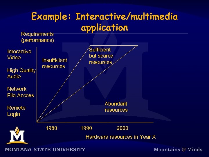Example: Interactive/multimedia application Requirements (performance) Interactive Video High Quality Audio Insufficient resources Sufficient but scarce resources Network File Access Abundant resources Remote Login 1980 1990 2000 Hardware resources in Year X

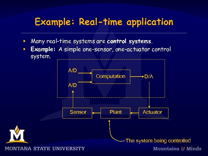Example: Real-time application § Many real-time systems are control systems. § Example: A simple one-sensor, one-actuator control system. A/D Computation D/A A/D Sensor Plant Actuator The system being controlled

Simple control system § Pseudo-code for this system: set timer to interrupt periodically with period T; at each timer interrupt do do analog-to-digital conversion to get y; compute control output u; output u and do digital-to-analog conversion; od § T is called the sampling period. T is a key design choice. Typical range for T: seconds to milliseconds.

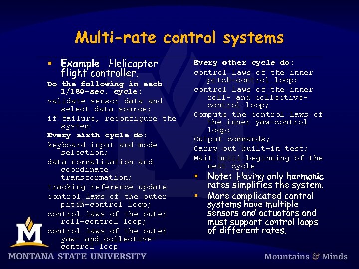Multi-rate control systems § Example Helicopter flight controller. Do the following in each 1/180 -sec. cycle: validate sensor data and select data source; if failure, reconfigure the system Every sixth cycle do: keyboard input and mode selection; data normalization and coordinate transformation; tracking reference update control laws of the outer pitch-control loop; control laws of the outer roll-control loop; control laws of the outer yaw- and collectivecontrol loop Every other cycle do: control laws of the inner pitch-control loop; control laws of the inner roll- and collectivecontrol loop; Compute the control laws of the inner yaw-control loop; Output commands; Carry out built-in test; Wait until beginning of the next cycle § § Note: Having only harmonic rates simplifies the system. More complicated control systems have multiple sensors and actuators and must support control loops of different rates.

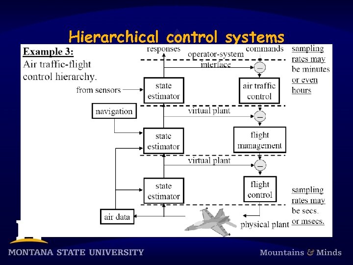Hierarchical control systems

Signal processing systems § Signal-processing systems transform data from one form to another. § Examples: § Digital filtering. § Video and voice compression/decompression. § Radar signal processing. § Response times range from a few milliseconds to a few seconds.

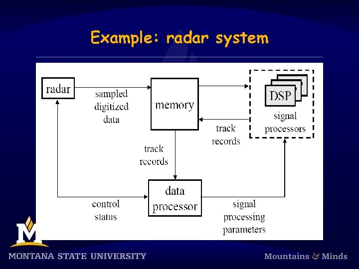Example: radar system

Other real-time applications § § Real-time databases. § Transactions must complete by deadlines. § Main dilemma: Transaction scheduling algorithms and real-time scheduling algorithms often have conflicting goals. § Data may be subject to absolute and relative temporal consistency requirements. Multimedia. § Want to process audio and video frames at steady rates. § TV video rate is 30 frames/sec. HDTV is 60 frames/sec. § Telephone audio is 16 Kbits/sec. CD audio is 128 Kbits/sec. § Other requirements: Lip synchronization, low jitter, low end-to -end response times (if interactive).

Hard vs. soft real-time § Task: A sequential piece of code. § Job: Instance of a task. § Jobs require resources to execute. § Example resources: CPU, network, disk, critical section. § We will simply call hardware resources “processors”. § Release time of a job: The time instant the job becomes ready to execute. § Deadline of a job: The time instant by which the job must complete execution. § Relative deadline of a job: “Deadline - Release time”. § Response time of a job: “Completion time - Release time”.

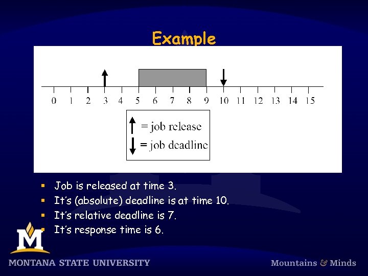Example § § Job is released at time 3. It’s (absolute) deadline is at time 10. It’s relative deadline is 7. It’s response time is 6.

Hard real-time systems § A hard deadline must be met. § If any hard deadline is ever missed, then the system is incorrect. § Requires a means for validating that deadlines are met. § Hard real-time system: A real-time system in which all deadlines are hard. § Examples: Nuclear power plant control, flight control.

Soft real-time systems § A soft deadline may occasionally be missed. § Question: How to define “occasionally”? § Soft real-time system: A real-time system in which some deadlines are soft. § Examples: Telephone switches, multimedia applications.

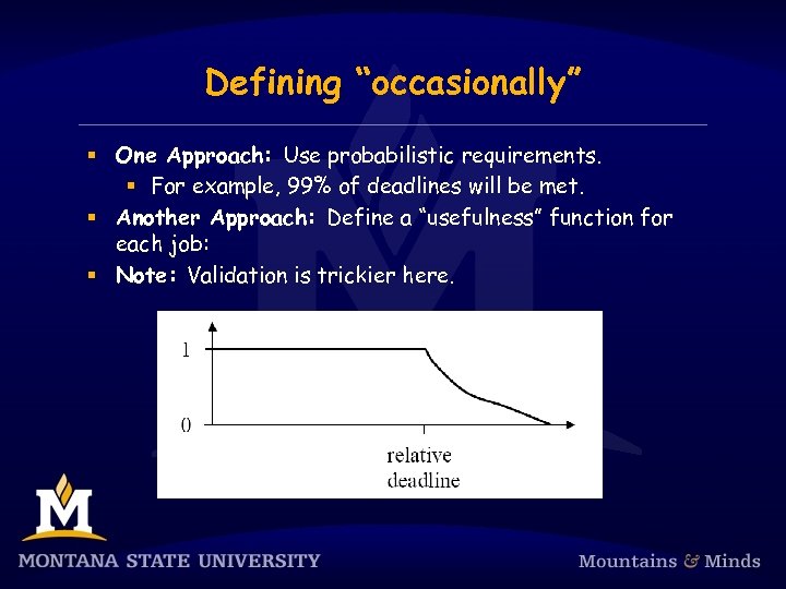Defining “occasionally” § One Approach: Use probabilistic requirements. § For example, 99% of deadlines will be met. § Another Approach: Define a “usefulness” function for each job: § Note: Validation is trickier here.

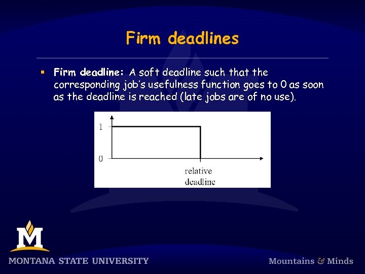Firm deadlines § Firm deadline: A soft deadline such that the corresponding job’s usefulness function goes to 0 as soon as the deadline is reached (late jobs are of no use).

Reference model § Each job Ji is characterized by its release time ri, absolute deadline di, relative deadline Di, and execution time ei. § Sometimes a range of release times is specified: [ri-, ri+]. This range is called release-time jitter. § Likewise, sometimes instead of ei, execution time is specified to range over [ei-, ei+]. § Note: It can be difficult to get a precise estimate of ei

Periodic, sporadic aperiodic tasks § Periodic task: § We associate a period pi with each task Ti. § pi is the time between job releases. § Sporadic and aperiodic tasks: Released at arbitrary times. § Sporadic: Has a hard deadline. § Aperiodic: Has no deadline or a soft deadline.

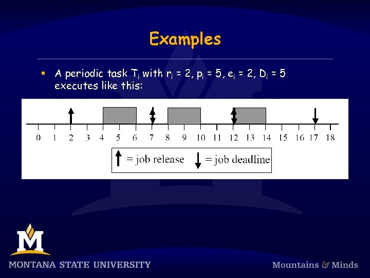Examples § A periodic task Ti with ri = 2, pi = 5, ei = 2, Di = 5 executes like this:

Some definitions for periodic task systems § The jobs of task Ti are denoted Ji, 1, Ji, 2, …. § ri, 1 (the release time of Ji, 1) is called the phase of Ti. § Synchronous System: Each task has a phase of 0. § Asynchronous System: Phases are arbitrary. § Hyperperiod: Least common multiple of {pi}. § Task utilization: ui = ei/pi. § System utilization: U = Σi=1. . nui.

Task dependencies § Two main kinds of dependencies: § Critical Sections. § Precedence Constraints. § For example, job Ji may be constrained to be released only after job Jk completes. § Tasks with no dependencies are called independent.

Scheduling algorithms § We are generally interested in two kinds of algorithms: 1. A scheduler or scheduling algorithm, which generates a schedule at runtime. 2. A feasibility analysis algorithm, which checks if timing constraints are met. § Usually (but not always) Algorithm 1 is pretty straightforward, while Algorithm 2 is more complex.

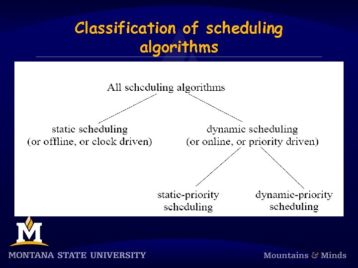Classification of scheduling algorithms

Optimality and feasibility § A schedule is feasible if all timing constraints are met. § The term “correct” is probably better — see the next slide. § A task set T is schedulable using scheduling algorithm A if A always produces a feasible schedule for T. § A scheduling algorithm is optimal if it always produces a feasible schedule when one exists (under any scheduling algorithm). § Can similarly define optimality for a class of schedulers, e. g. , “an optimal static-priority scheduling algorithm. ”

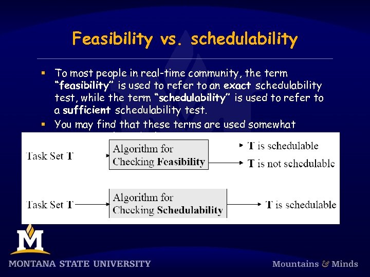Feasibility vs. schedulability § To most people in real-time community, the term “feasibility” is used to refer to an exact schedulability test, while the term “schedulability” is used to refer to a sufficient schedulability test. § You may find that these terms are used somewhat inconsistently in the literature.

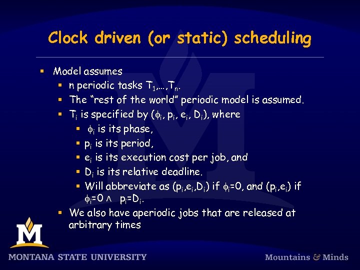Clock driven (or static) scheduling § Model assumes § n periodic tasks T 1, …, Tn. § The “rest of the world” periodic model is assumed. § Ti is specified by (fi, pi, ei, Di), where § fi is its phase, § pi is its period, § ei is its execution cost per job, and § Di is its relative deadline. § Will abbreviate as (pi, ei, Di) if fi=0, and (pi, ei) if fi=0 ∧ pi=Di. § We also have aperiodic jobs that are released at arbitrary times

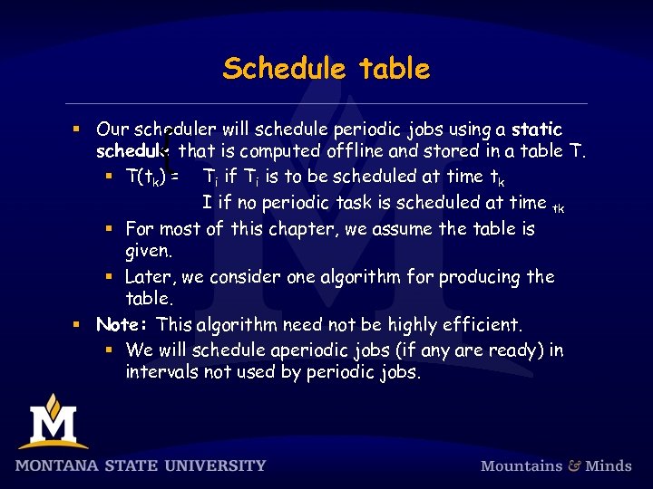Schedule table { § Our scheduler will schedule periodic jobs using a static schedule that is computed offline and stored in a table T. § T(tk) = Ti if Ti is to be scheduled at time tk I if no periodic task is scheduled at time tk § For most of this chapter, we assume the table is given. § Later, we consider one algorithm for producing the table. § Note: This algorithm need not be highly efficient. § We will schedule aperiodic jobs (if any are ready) in intervals not used by periodic jobs.

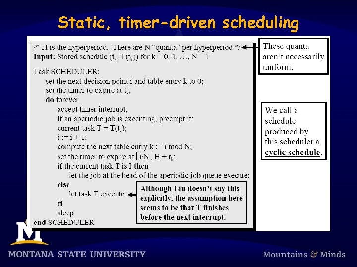Static, timer-driven scheduling

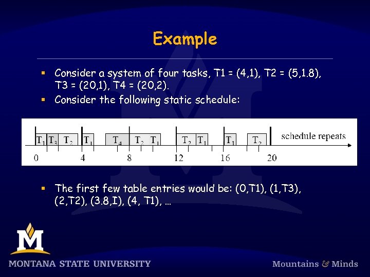Example § Consider a system of four tasks, T 1 = (4, 1), T 2 = (5, 1. 8), T 3 = (20, 1), T 4 = (20, 2). § Consider the following static schedule: § The first few table entries would be: (0, T 1), (1, T 3), (2, T 2), (3. 8, I), (4, T 1), …

Frames § Let us refine this notion of scheduling… § To keep the table small, we divide the time line into frames and make scheduling decisions only at frame boundaries. § Each job is executed as a procedure call that must fit within a frame. § Multiple jobs may be executed in a frame, but the table is only examined at frame boundaries (the number of “columns” in the table = the number of frames per hyperperiod). § In addition to making scheduling decisions, the scheduler also checks for various error conditions, like task overruns, at the beginning of each frame. § We let f denote the frame size.

Frame size constraints § We want frames to be sufficiently long so that every job can execute within a frame nonpreemptively. So, § f ³ max 1£i£n(ei). § To keep table small, f should divide H. Thus, for at least one task Ti, ëpi/fû - pi/f = 0. § Let F = H/f. (Note: F is an integer. ) Each interval of length H is called a major cycle. Each interval of length f is called a minor cycle. § There are F minor cycles per major cycle.

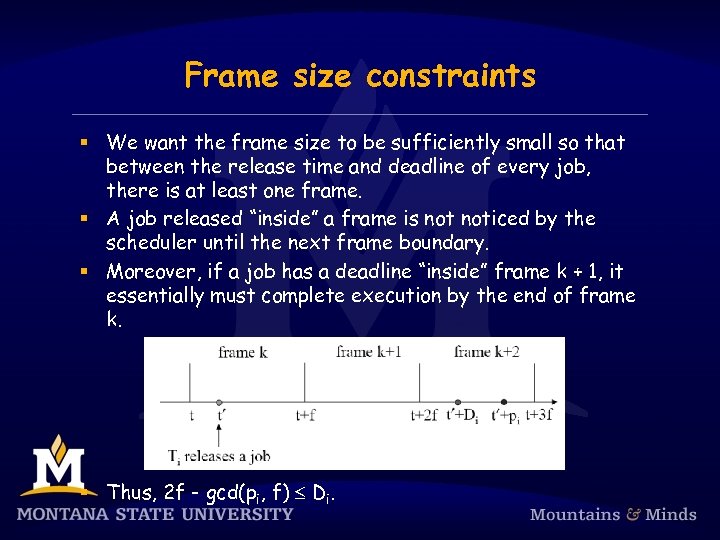Frame size constraints § We want the frame size to be sufficiently small so that between the release time and deadline of every job, there is at least one frame. § A job released “inside” a frame is noticed by the scheduler until the next frame boundary. § Moreover, if a job has a deadline “inside” frame k + 1, it essentially must complete execution by the end of frame k. § Thus, 2 f - gcd(pi, f) £ Di.

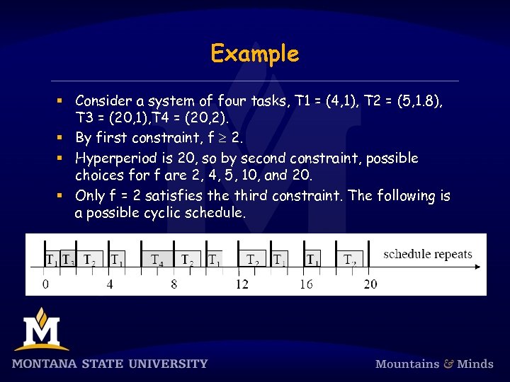Example § Consider a system of four tasks, T 1 = (4, 1), T 2 = (5, 1. 8), T 3 = (20, 1), T 4 = (20, 2). § By first constraint, f ³ 2. § Hyperperiod is 20, so by second constraint, possible choices for f are 2, 4, 5, 10, and 20. § Only f = 2 satisfies the third constraint. The following is a possible cyclic schedule.

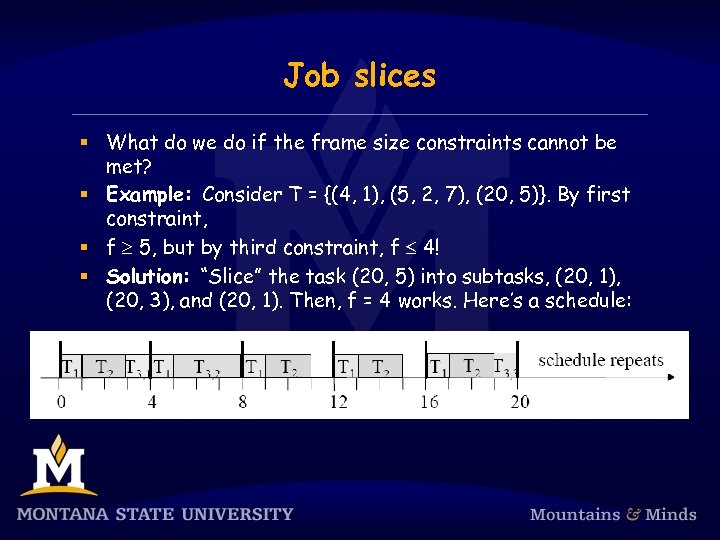Job slices § What do we do if the frame size constraints cannot be met? § Example: Consider T = {(4, 1), (5, 2, 7), (20, 5)}. By first constraint, § f ³ 5, but by third constraint, f £ 4! § Solution: “Slice” the task (20, 5) into subtasks, (20, 1), (20, 3), and (20, 1). Then, f = 4 works. Here’s a schedule:

Summary of design decisions § Three design decisions: § choosing a frame size, § partitioning jobs into slices, and § placing slices in frames. § In general, these decisions cannot be made independently.

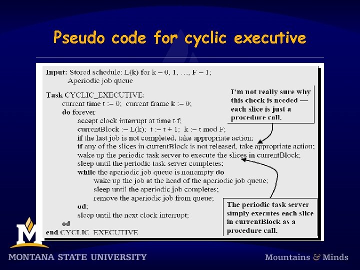Pseudo code for cyclic executive

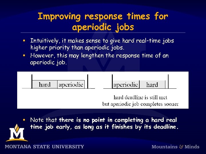Improving response times for aperiodic jobs § Intuitively, it makes sense to give hard real-time jobs higher priority than aperiodic jobs. § However, this may lengthen the response time of an aperiodic job. § Note that there is no point in completing a hard real time job early, as long as it finishes by its deadline.

Slack stealing § Let the total amount of time allocated to all the slices scheduled in frame k be xk. § Definition: The slack available at the beginning of frame k is f - xk. § Change to scheduler: § If the aperiodic job queue is non-empty, let aperiodic jobs execute in each frame whenever there is nonzero slack.

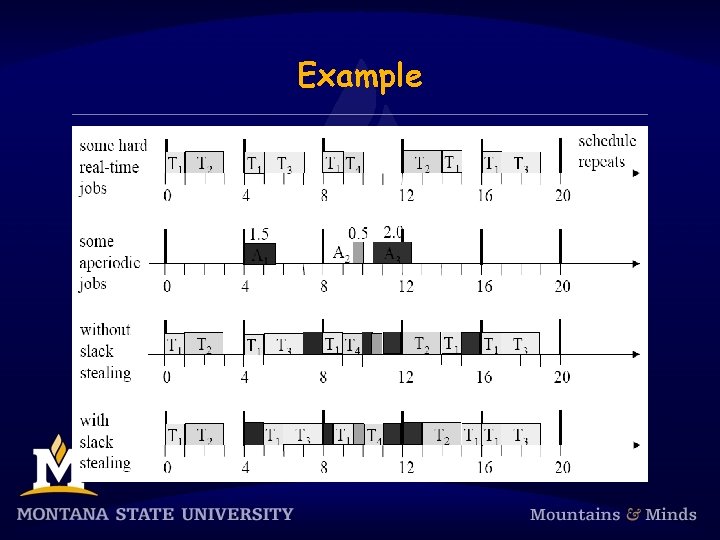Example

Implementing slack stealing § Use a pre-computed “initial slack” table. § Initial slack depends only on static quantities. § Use an interval timer to keep track of available slack. § Set the timer when an aperiodic job begins to run. If it goes off, must start executing periodic jobs. § Problem: Most OSs do not provide sub-millisecond granularity interval timers. § So, to use slack stealing, temporal parameters must be on the order of 100 s of msecs. or secs.

Scheduling sporiadic jobs Sporadic jobs arrive at arbitrary times. They have hard deadlines. Implies we cannot hope to schedule every sporadic job. When a sporadic job arrives, the scheduler performs an acceptance test to see if the job can be completed by its deadline. § We must ensure that a new sporadic job does not cause a previously-accepted sporadic job to miss its deadline. § We assume sporadic jobs are prioritized on an earliest deadline- first (EDF) basis. § §

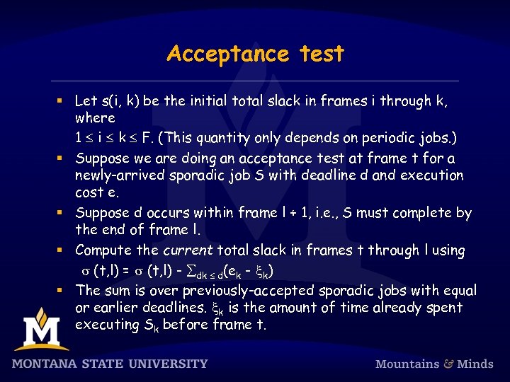Acceptance test § Let s(i, k) be the initial total slack in frames i through k, where 1 £ i £ k £ F. (This quantity only depends on periodic jobs. ) § Suppose we are doing an acceptance test at frame t for a newly-arrived sporadic job S with deadline d and execution cost e. § Suppose d occurs within frame l + 1, i. e. , S must complete by the end of frame l. § Compute the current total slack in frames t through l using s (t, l) = s (t, l) - ådk £ d(ek - xk) § The sum is over previously-accepted sporadic jobs with equal or earlier deadlines. xk is the amount of time already spent executing Sk before frame t.

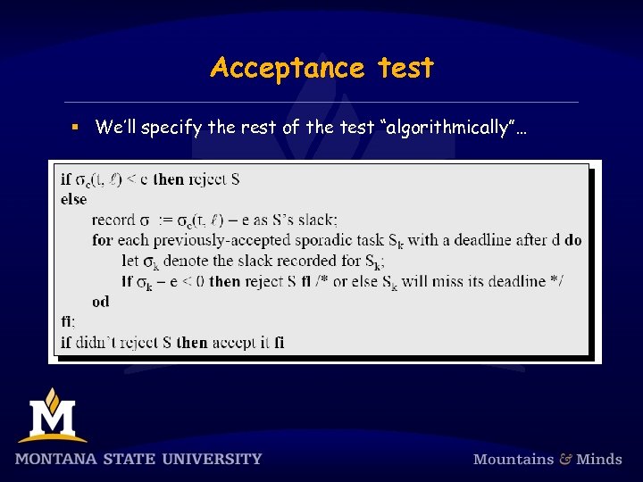Acceptance test § We’ll specify the rest of the test “algorithmically”…

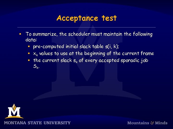Acceptance test § To summarize, the scheduler must maintain the following data: § pre-computed initial slack table s(i, k); § xk values to use at the beginning of the current frame § the current slack sk of every accepted sporadic job Sk.

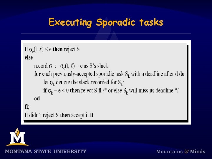Executing Sporadic tasks

Executing sporadic tasks § Accepted sporadic jobs are executed like aperiodic obs in the original alg. (without slack stealing). § Remember, when meeting a deadline is the main concern, there is no need to complete a job early. § One difference: The aperiodic job queue is in FIFO order, while the sporadic job queue is in EDF order. § Aperiodic jobs only execute when the sporadic job queue is empty. § As before, slack stealing could be used when executing aperiodic jobs (in which case, some aperiodic jobs could execute when the sporadic job queue is not empty).

Practical considerations § Handling frame overruns. § Main Issue: Should offending job be completed or aborted? § Mode changes. § During a mode change, the running set of tasks is replaced by a new set of tasks (i. e. , the table is changed). § Can implement mode change by having an aperiodic or sporadic mode-change job. (If sporadic, what if it fails the acceptance test? ? ? ) § Multiprocessors. § Like uniprocessors, but table probably takes longer to precompute.

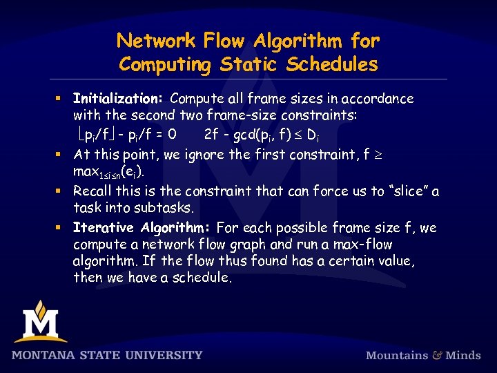Network Flow Algorithm for Computing Static Schedules § Initialization: Compute all frame sizes in accordance with the second two frame-size constraints: ëpi/fû - pi/f = 0 2 f - gcd(pi, f) £ Di § At this point, we ignore the first constraint, f ³ max 1£i£n(ei). § Recall this is the constraint that can force us to “slice” a task into subtasks. § Iterative Algorithm: For each possible frame size f, we compute a network flow graph and run a max-flow algorithm. If the flow thus found has a certain value, then we have a schedule.

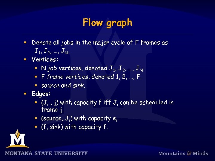Flow graph § Denote all jobs in the major cycle of F frames as J 1, J 2, …, JN. § Vertices: § N job vertices, denoted J 1, J 2, …, JN. § F frame vertices, denoted 1, 2, …, F. § source and sink. § Edges: § (Ji , j) with capacity f iff Ji can be scheduled in frame j. § (source, Ji) with capacity ei. § (f, sink) with capacity f.

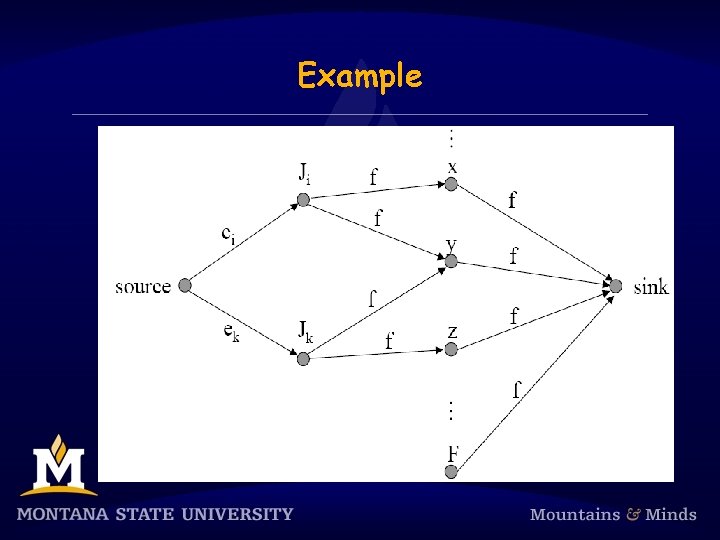Example

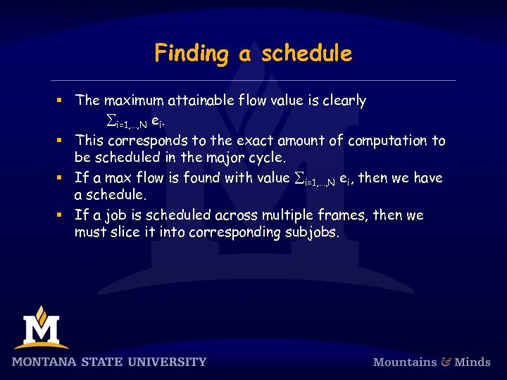Finding a schedule § The maximum attainable flow value is clearly åi=1, …, N ei. § This corresponds to the exact amount of computation to be scheduled in the major cycle. § If a max flow is found with value åi=1, …, N ei, then we have a schedule. § If a job is scheduled across multiple frames, then we must slice it into corresponding subjobs.

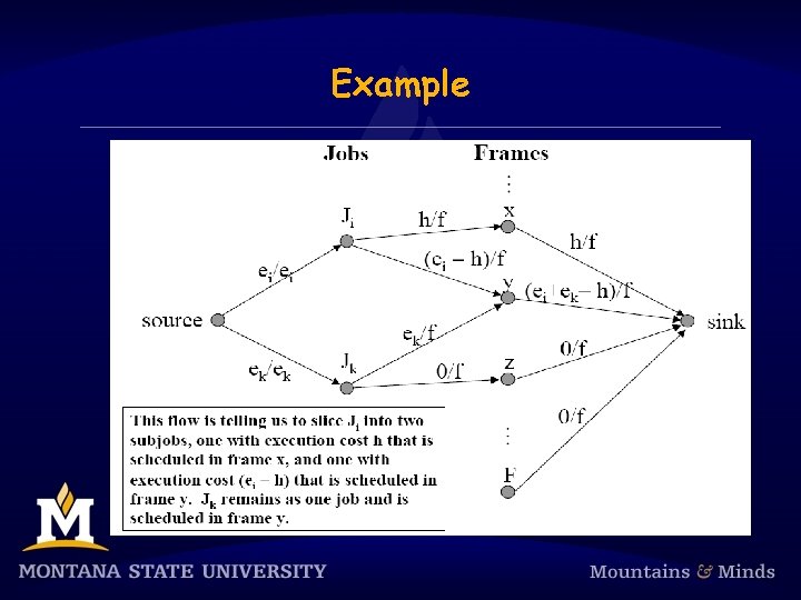Example

Non-independent tasks § Tasks with precedence constraints are no problem. § We can enforce precedence constraint like “Ji precedes Jk” by simply making sure Ji’s release is at or before Jk’s release, and Ji’s deadline is at or before Jk’s deadline. § If slices of Ji and Jk are scheduled in the wrong order, we can just swap them. § Critical sections pose a greater challenge. § We can try to “massage” the flow-network schedule into one where nonpreemption constraints are respected. § Unfortunately, there is no known efficient, optimal algorithm for doing this (the problem is actually NPhard).

Pros and Cons of Cyclic Executives § Main Advantage: CEs are very simple - you just need a table. § For example, additional mechanisms for concurrency control and synchronization are not needed. In fact, there’s really no notion of a “process” here – just procedure calls. § Can validate, test, and certify with very high confidence. § Certain anomalies will not occur. § For these reasons, cyclic executives are the predominant approach in many safety-critical applications (like airplanes).

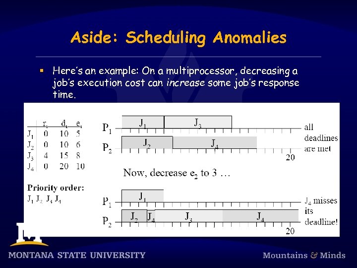Aside: Scheduling Anomalies § Here’s an example: On a multiprocessor, decreasing a job’s execution cost can increase some job’s response time. § Example: Suppose we have one job queue, preemption, but no migration.

Disadvantages § Disadvantages of cyclic executives: § Very brittle: Any change, no matter how trivial, requires that a new table be computed! § Release times of all jobs must be fixed, i. e. , “real-world” sporadic tasks are difficult to support. § Temporal parameters essentially must be multiples of f. § F could be huge! § All combinations of periodic tasks that may execute together must a priori be analyzed. § From a software engineering standpoint, “slicing” one procedure into several could be error-prone.

Dynamic-priority scheduling § Let us consider a priority-based dynamic scheduling approach. § Each job is assigned a priority, and the highestpriority job executes at any time. § Under dynamic-priority scheduling, different jobs of a task may be assigned different priorities. § Can have the following: job Ji, k of task Ti has higher priority than job Jj, m of task Tj, but job Ji, l of Ti has lower priority than job Jj, n of Tj.

Outline § We consider both earliest-deadline-first (EDF) and least-laxity-first (LLF) scheduling. § Outline: § Optimality of EDF and LLF § Utilization-based schedulability test for EDF

Optimality of EDF § Theorem: [Liu and Layland] When preemption is allowed and jobs do not contend for resources, the EDF algorithm can produce a feasible schedule of a set J of independent jobs with arbitrary release times and deadlines on a processor if and only if J has feasible schedules. § Notes: § Applies even if tasks are not periodic. § If periodic, a task’s relative deadline can be less than its period, equal to its period, or greater than its period.

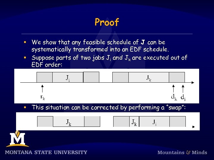Proof § We show that any feasible schedule of J can be systematically transformed into an EDF schedule. § Suppose parts of two jobs Ji and Jk are executed out of EDF order: § This situation can be corrected by performing a “swap”:

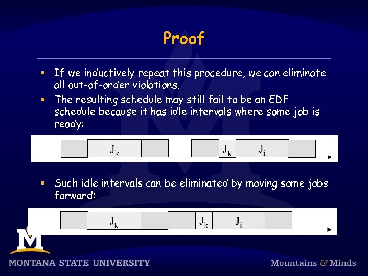Proof § If we inductively repeat this procedure, we can eliminate all out-of-order violations. § The resulting schedule may still fail to be an EDF schedule because it has idle intervals where some job is ready: § Such idle intervals can be eliminated by moving some jobs forward:

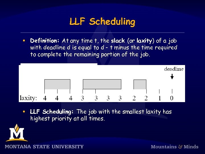LLF Scheduling § Definition: At any time t, the slack (or laxity) of a job with deadline d is equal to d - t minus the time required to complete the remaining portion of the job. § LLF Scheduling: The job with the smallest laxity has highest priority at all times.

Optimality of LLF § Theorem: When preemption is allowed and jobs do not contend for resources, the LLF algorithm can produce a feasible schedule of a set J of independent jobs with arbitrary release times and deadlines on a processor if and only if J has feasible schedules. § The proof is similar to that for EDF.