Real Options Life wasn t designed to be risk-free

Real Options “Life wasn’t designed to be risk-free. The key is not to eliminate, but to estimate it accurately and manage it wisely. ” -William Schreyer, former Chair and CEO of Merrill Lynch

Options Are Everywhere! • • Callable Bonds Convertible Securities Warrants Secure Loans Firm with Debt Exotics Compensation Real Options 2

Real versus Financial Options • Transparency • Information • Contract details • Valuation? 3

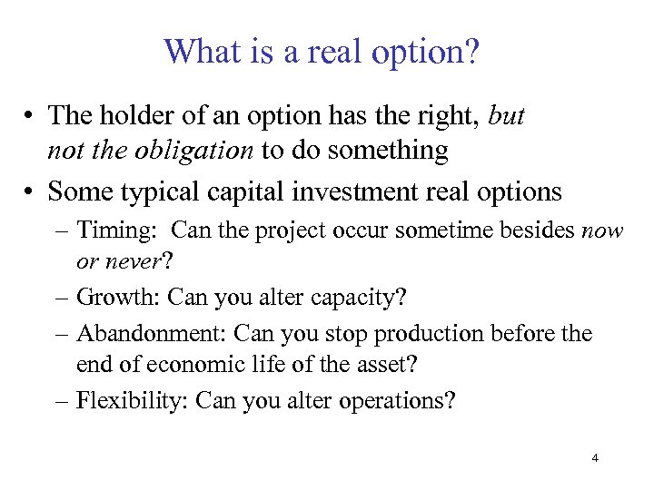
What is a real option? • The holder of an option has the right, but not the obligation to do something • Some typical capital investment real options – Timing: Can the project occur sometime besides now or never? – Growth: Can you alter capacity? – Abandonment: Can you stop production before the end of economic life of the asset? – Flexibility: Can you alter operations? 4

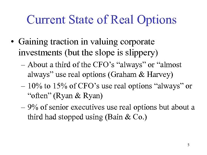
Current State of Real Options • Gaining traction in valuing corporate investments (but the slope is slippery) – About a third of the CFO’s “always” or “almost always” use real options (Graham & Harvey) – 10% to 15% of CFO’s use real options “always” or “often” (Ryan & Ryan) – 9% of senior executives use real options but about a third had stopped using (Bain & Co. ) 5

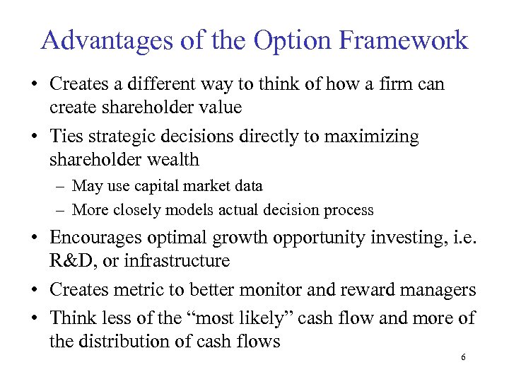
Advantages of the Option Framework • Creates a different way to think of how a firm can create shareholder value • Ties strategic decisions directly to maximizing shareholder wealth – May use capital market data – More closely models actual decision process • Encourages optimal growth opportunity investing, i. e. R&D, or infrastructure • Creates metric to better monitor and reward managers • Think less of the “most likely” cash flow and more of the distribution of cash flows 6

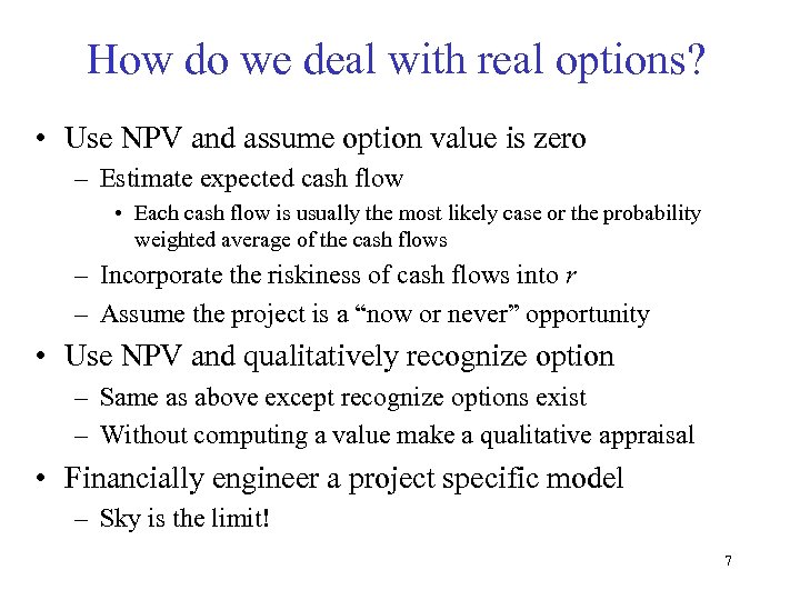
How do we deal with real options? • Use NPV and assume option value is zero – Estimate expected cash flow • Each cash flow is usually the most likely case or the probability weighted average of the cash flows – Incorporate the riskiness of cash flows into r – Assume the project is a “now or never” opportunity • Use NPV and qualitatively recognize option – Same as above except recognize options exist – Without computing a value make a qualitative appraisal • Financially engineer a project specific model – Sky is the limit! 7

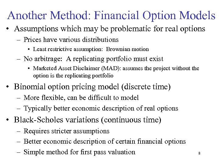
Another Method: Financial Option Models • Assumptions which may be problematic for real options – Prices have various distributions • Least restrictive assumption: Brownian motion – No arbitrage: A replicating portfolio must exist • Marketed Asset Disclaimer (MAD): assumes the project without the option is the replicating portfolio • Binomial option pricing model (discrete time) – More flexible, can be difficult to model – Typically better economic description of real options • Black-Scholes variations (continuous time) – Requires stricter assumptions – Better economic description of certain financial options – Simple method for first pass valuation 8

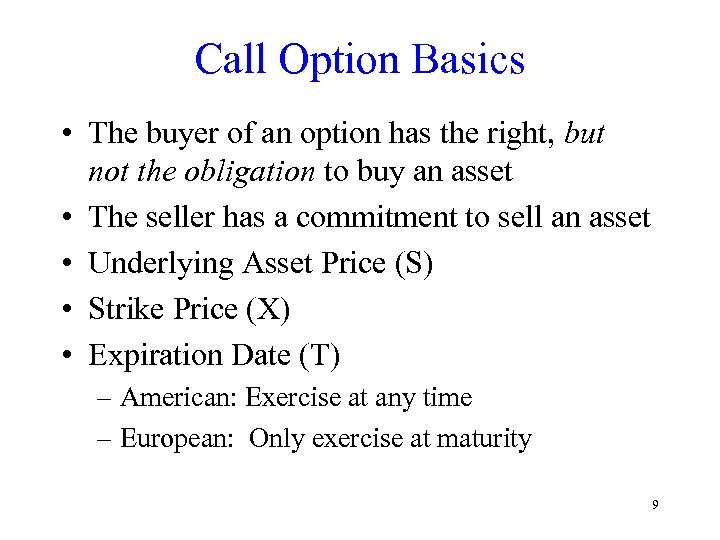
Call Option Basics • The buyer of an option has the right, but not the obligation to buy an asset • The seller has a commitment to sell an asset • Underlying Asset Price (S) • Strike Price (X) • Expiration Date (T) – American: Exercise at any time – European: Only exercise at maturity 9

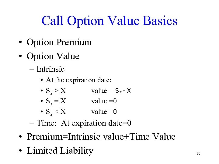
Call Option Value Basics • Option Premium • Option Value – Intrinsic • • At the expiration date: ST > X value = ST - X ST = X value =0 ST < X value =0 – Time: At expiration date=0 • Premium=Intrinsic value+Time Value • Limited Liability 10

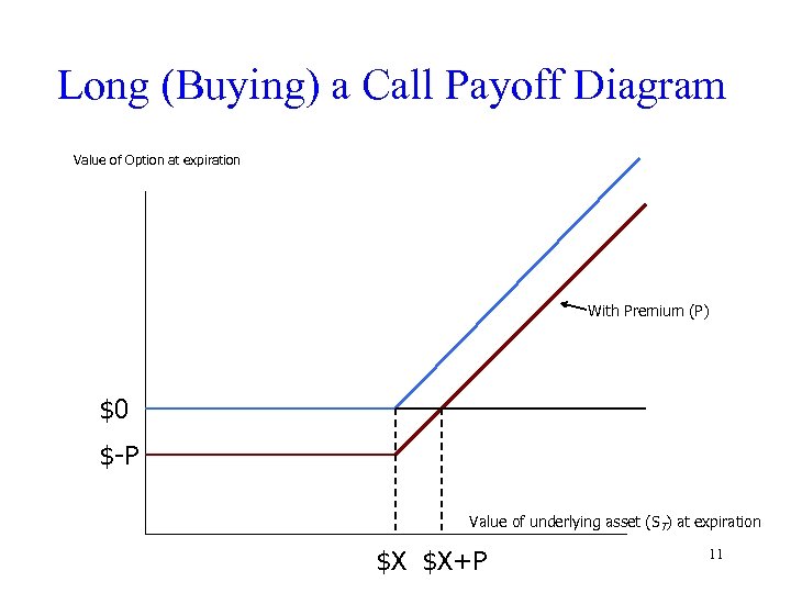
Long (Buying) a Call Payoff Diagram Value of Option at expiration With Premium (P) $0 $-P Value of underlying asset (ST) at expiration $X $X+P 11

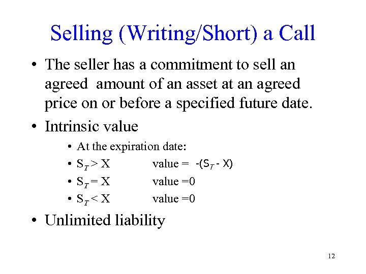
Selling (Writing/Short) a Call • The seller has a commitment to sell an agreed amount of an asset at an agreed price on or before a specified future date. • Intrinsic value • • At the expiration date: ST > X value = -(ST - X) ST = X value =0 ST < X value =0 • Unlimited liability 12

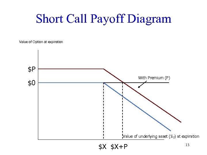
Short Call Payoff Diagram Value of Option at expiration $P With Premium (P) $0 Value of underlying asset (ST) at expiration $X $X+P 13

Buying Versus Selling • Liability • Obligation versus Commitment 14

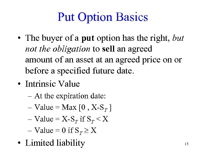
Put Option Basics • The buyer of a put option has the right, but not the obligation to sell an agreed amount of an asset at an agreed price on or before a specified future date. • Intrinsic Value – At the expiration date: – Value = Max [0 , X-ST ] – Value = X-ST if ST < X – Value = 0 if ST X • Limited liability 15

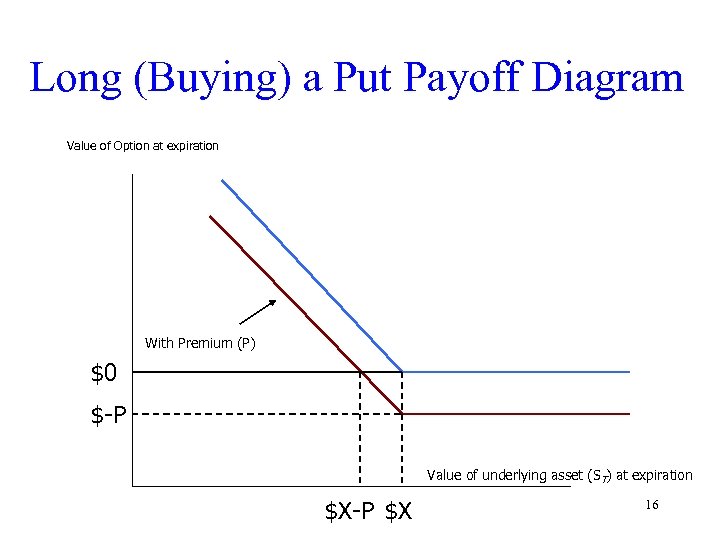
Long (Buying) a Put Payoff Diagram Value of Option at expiration With Premium (P) $0 $-P Value of underlying asset (ST) at expiration $X-P $X 16

Selling a Put • The buyer of a put option has the right, but not the obligation to sell an asset • The seller has a commitment to buy an asset. • Intrinsic value – At the expiration date: – Value = -(X-ST ) if ST < X – Value = 0 if ST X • Unlimited liability 17

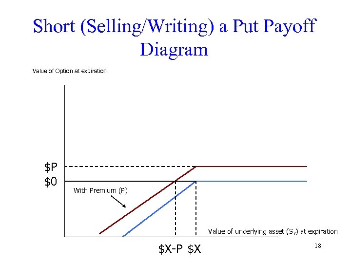
Short (Selling/Writing) a Put Payoff Diagram Value of Option at expiration $P $0 With Premium (P) Value of underlying asset (ST) at expiration $X-P $X 18

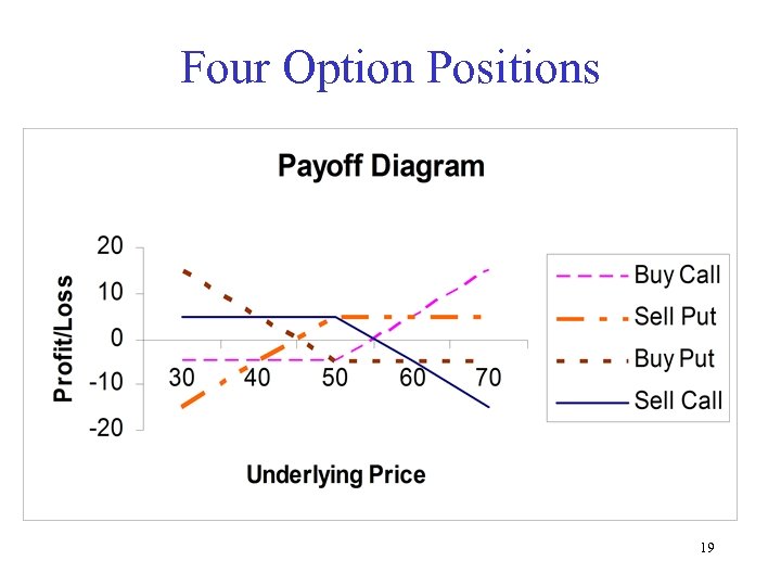
Four Option Positions 19

Valuation Basics 20

How Do We Value? • Option Value=Intrinsic+Time • Focus on Time Component – Time till Maturity (T) • What if the call option is out of the money? • Near the money? • In the money? – Exercise before expiration? – S 0 -PV(X) 21

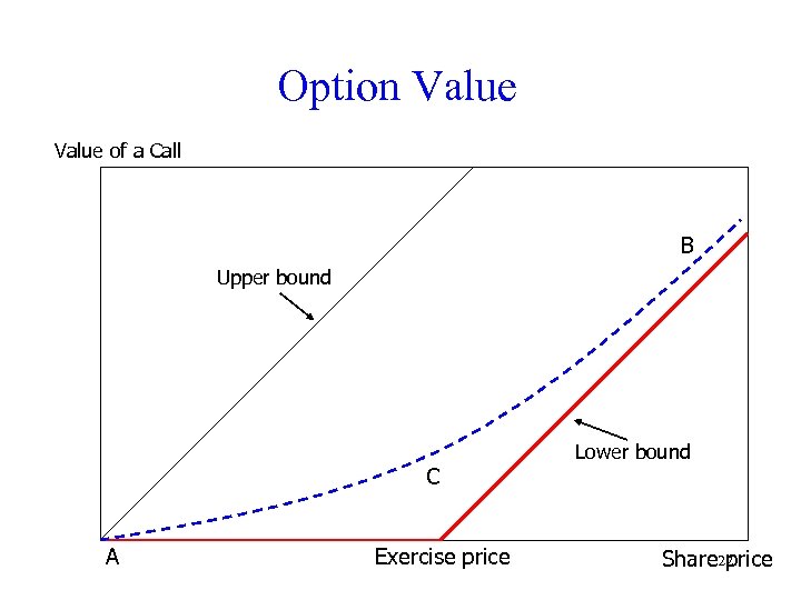
Option Value of a Call B Upper bound C A Exercise price Lower bound Share 22 price

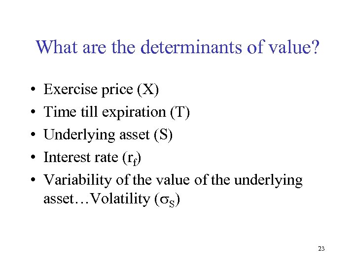
What are the determinants of value? • • • Exercise price (X) Time till expiration (T) Underlying asset (S) Interest rate (rf) Variability of the value of the underlying asset…Volatility ( S) 23

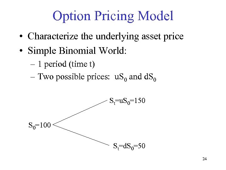
Option Pricing Model • Characterize the underlying asset price • Simple Binomial World: – 1 period (time t) – Two possible prices: u. S 0 and d. S 0 St=u. S 0=150 S 0=100 St=d. S 0=50 24

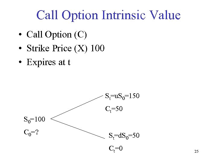
Call Option Intrinsic Value • Call Option (C) • Strike Price (X) 100 • Expires at t St=u. S 0=150 Ct=50 S 0=100 C 0=? St=d. S 0=50 Ct=0 25

What is the value of the call today? • Assumption: No Arbitrage Opportunities • Establish an arbitrage portfolio of the option and underlying asset – This portfolio has a constant return – What is that return? • Portfolio – Short Call – Long stock 26

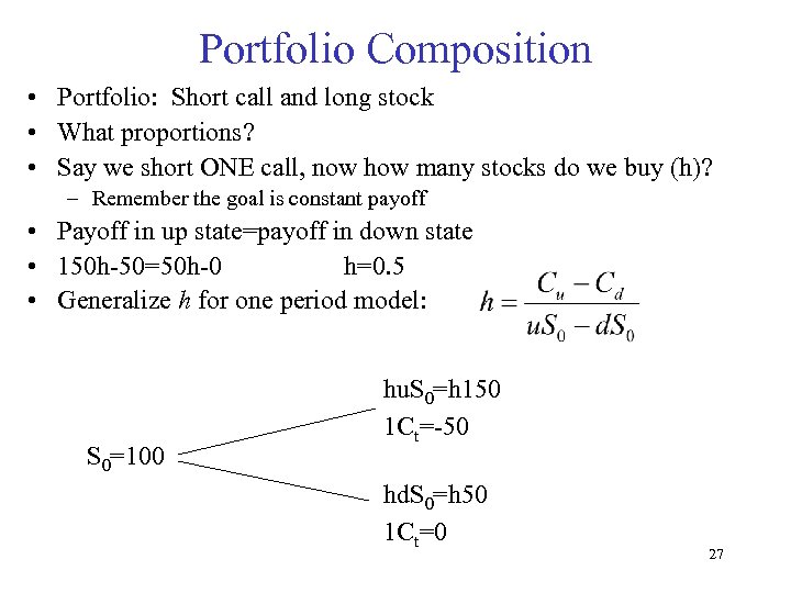
Portfolio Composition • Portfolio: Short call and long stock • What proportions? • Say we short ONE call, now how many stocks do we buy (h)? – Remember the goal is constant payoff • Payoff in up state=payoff in down state • 150 h-50=50 h-0 h=0. 5 • Generalize h for one period model: S 0=100 hu. S 0=h 150 1 Ct=-50 hd. S 0=h 50 1 Ct=0 27

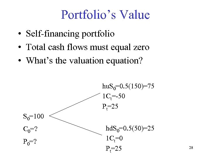
Portfolio’s Value • Self-financing portfolio • Total cash flows must equal zero • What’s the valuation equation? hu. S 0=0. 5(150)=75 1 Ct=-50 Pt=25 S 0=100 C 0=? P 0=? hd. S 0=0. 5(50)=25 1 Ct=0 Pt=25 28

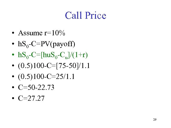
Call Price • • Assume r=10% h. S 0 -C=PV(payoff) h. S 0 -C=[hu. S 0 -Cu]/(1+r) (0. 5)100 -C=[75 -50]/1. 1 (0. 5)100 -C=25/1. 1 C=50 -22. 73 C=27. 27 29

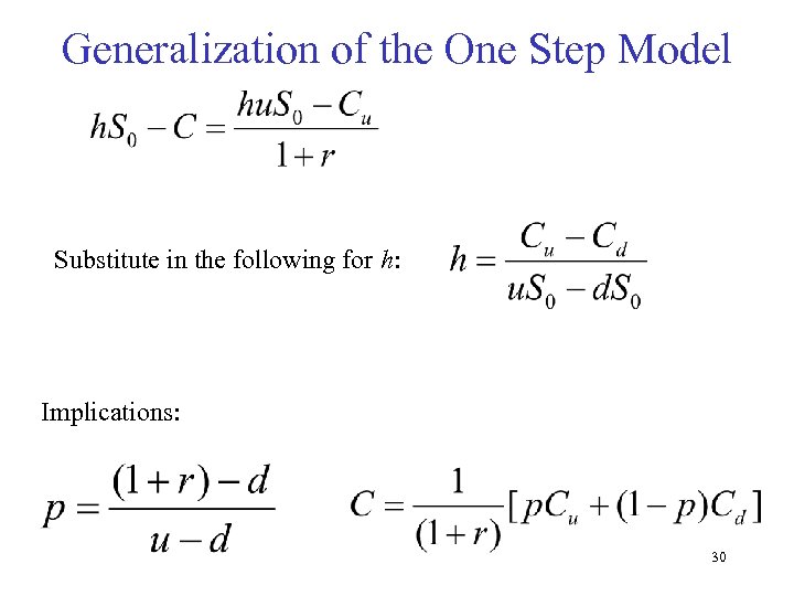
Generalization of the One Step Model Substitute in the following for h: Implications: 30

Important Characteristics • Backward induction method – Rollback values one period at a time • Arbitrage portfolio guarantees that the payoff is identical in all states of nature – No longer concerned which path the price on the underlying asset takes – Implies that you are not concerned about state dependent risk – Implies that all investors are risk neutral • Used in all derivatives pricing • Simplifying assumption – What is the appropriate r? • The risk free rate! 31

Risk Neutral Valuation • Investors are risk-neutral (the probability of underlying asset moves don’t matter), they require 10% • The share price can increase/decrease by 50% • What is the probability of an increase/decrease? – – – p=[(1+r)-d]/(u-d)=[1. 1 -0. 5]/(1. 5 -0. 5)=0. 6 Intuitively: 1+0. 1 = P(increase) × 1. 5 + P(decrease) × 0. 5 1. 1 = P(increase) × 1. 5 + P(1 - increase) × 0. 5 P(increase) =60% and P(decrease)=40% (Risk-neutral probabilities) • Given the call prices for the two scenarios: – [1/1. 1] x [p. Cu+(1 -p)Cd] – [1/1. 1] x [0. 60 × $50 + 0. 40 × $0] = $27. 27 32

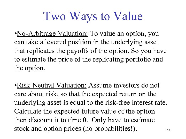
Two Ways to Value • No-Arbitrage Valuation: To value an option, you can take a levered position in the underlying asset that replicates the payoffs of the option. So you have to estimate the price of the replicating portfolio and the option. • Risk-Neutral Valuation: Assume investors do not care about risk, so that the expected return on the underlying asset is equal to the risk-free interest rate. Calculate the expected future value of the option then discount it to time 0. Only have to estimate stock and option prices (no probabilities!). 33

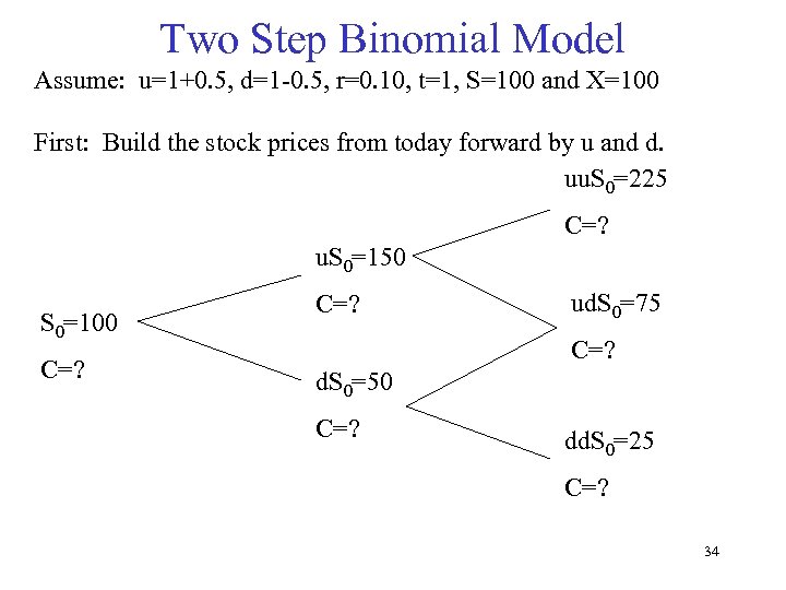
Two Step Binomial Model Assume: u=1+0. 5, d=1 -0. 5, r=0. 10, t=1, S=100 and X=100 First: Build the stock prices from today forward by u and d. uu. S 0=225 C=? u. S 0=150 S 0=100 C=? ud. S 0=75 C=? d. S 0=50 C=? dd. S 0=25 C=? 34

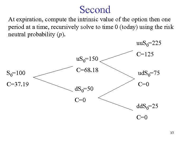
Second At expiration, compute the intrinsic value of the option then one period at a time, recursively solve to time 0 (today) using the risk neutral probability (p). uu. S 0=225 u. S 0=150 S 0=100 C=37. 19 C=68. 18 d. S 0=50 C=125 ud. S 0=75 C=0 dd. S 0=25 C=0 35

Valuing a Put • Remember: Intrinsic value of a put is Max[0, X-ST] • Intuitively, what is different for a put – Underlying stock price? • No difference – At maturity payoff (intrinsic value)? • Max [0, X-ST] instead of Max[0, ST-X] – Recursive solution • Risk neutral probability (p)? – No difference • Put computation (C=)? – No difference 36

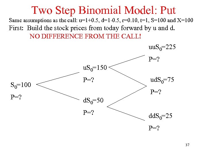
Two Step Binomial Model: Put Same assumptions as the call: u=1+0. 5, d=1 -0. 5, r=0. 10, t=1, S=100 and X=100 First: Build the stock prices from today forward by u and d. NO DIFFERENCE FROM THE CALL! uu. S 0=225 P=? u. S 0=150 S 0=100 P=? ud. S 0=75 P=? d. S 0=50 P=? dd. S 0=25 P=? 37

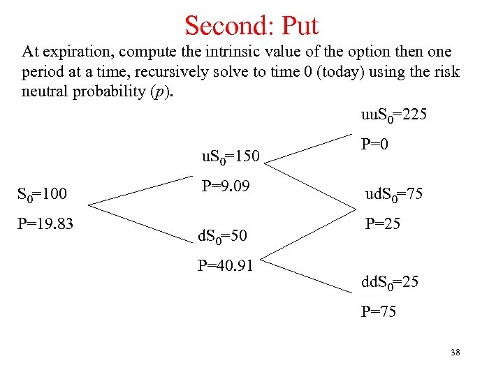
Second: Put At expiration, compute the intrinsic value of the option then one period at a time, recursively solve to time 0 (today) using the risk neutral probability (p). uu. S 0=225 u. S 0=150 S 0=100 P=19. 83 P=9. 09 d. S 0=50 P=40. 91 P=0 ud. S 0=75 P=25 dd. S 0=25 P=75 38

Valuing an American Option • Remember an American option can be exercised any time before (or at) maturity – European option can only be exercised at maturity • Intuitively, what is the difference? – Underlying stock price? • No difference – At maturity payoff? • No difference – Backward induction • Risk neutral probability (p)? – No difference • Put or Call computation – Partial difference: The same except at each node, take the higher of the option value or the exercise price (C=S-X, P=X-S) 39

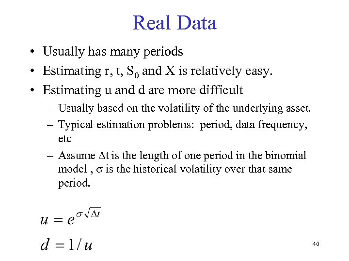
Real Data • Usually has many periods • Estimating r, t, S 0 and X is relatively easy. • Estimating u and d are more difficult – Usually based on the volatility of the underlying asset. – Typical estimation problems: period, data frequency, etc – Assume Dt is the length of one period in the binomial model , is the historical volatility over that same period. 40

Option Delta • How many shares are needed to replicate an option? • Option Delta = Spread of Possible Option Prices / Spread of Possible Share Prices – Delta = (125 - 0) / (225 - 25)= 5/8 • Delta of a Put = Delta of a Call with the same exercise price minus 1 41

Black-Scholes versus Binomial Model • Continuous versus Discrete Time – Assume stock price can be characterized by a continuous process • Special limiting case of Binomial as the length of the period approaches zero • Computationally easier • More restrictive assumptions • Several variations to account for different types of underlying assets 42

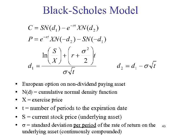
Black-Scholes Model • European option on non-dividend paying asset • N(d) = cumulative normal density function • X = exercise price • t = number of periods to the expiration date • S = current stock price (underlying asset) • = standard deviation period of the rate of return on the underlying asset (continuously compounded) 43

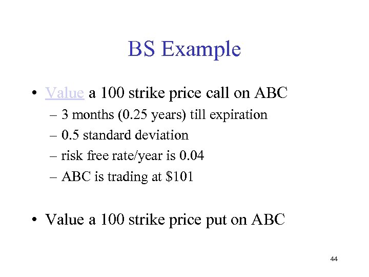
BS Example • Value a 100 strike price call on ABC – 3 months (0. 25 years) till expiration – 0. 5 standard deviation – risk free rate/year is 0. 04 – ABC is trading at $101 • Value a 100 strike price put on ABC 44

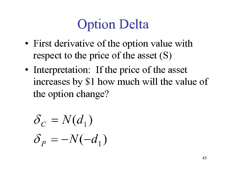
Option Delta • First derivative of the option value with respect to the price of the asset (S) • Interpretation: If the price of the asset increases by $1 how much will the value of the option change? 45

Black-Scholes Variations • American options on non-dividend paying assets • European options on assets that have – discrete (point in time before expiration) dividend – continuous proportion dividend such as index futures • European options on foreign currency • European options on futures and forwards • Etc. 46

DCF to Real Options • Exercise Price (X)? – Initial investment (investment required to acquire the assets) • Underlying asset (S)? – PV (CF) excluding initial investment (value of the operating assets to be acquired) • Time to expiration (t)? – Length of time the choice is available • Volatility ( )? – Riskiness of underlying operating assets • Risk free rate? – Time value of money: If replicating portfolio exists the risk free rate. If not, the risk free rate will provide the upper bound. 47

DCF versus Real Options • One method does not completely dominate – Both methods used correctly will give identical values – Each method frames the question differently • DCF – Works well for “assets in place” type of projects – Lower uncertainty, less decision nodes • Real Options – Works well for “growth option” type of projects – Greater span of possible cash flows, many decision nodes 48