Real Options An Intuitive Introduction and Simple Applications

Real Options An Intuitive Introduction and Simple Applications Dr. C. Bülent Aybar Professor of International Finance

Traditional NPV Method • The NPV rule implicitly assumes a “buy and hold” strategy, where the analyst’s best guess of future net cash flows attributable to the investment are discounted to present values. • The risk of these cash flows is incorporated in the discounting procedure through a riskadjusted discount rate.

• Traditional NPV criterion does a reasonable job of valuing simple, passively managed projects; • However, it does not capture the many ways a highly uncertain project might evolve, and the ways in which active managers will influence this evolution!

A Simple Example • A pharmaceutical firm’s research and development program recently generated a promising idea for a new pharmaceutical product, and successful Phase II clinical trials of the drug have just been completed. • One year of Phase III clinical trials is now required. If the trials lead to FDA approval for an indication with broad market potential, they will be followed by full-scale production. • Capital outlays are required to begin the trials, and a much larger expenditure will be required one year from now as mass production is initiated.

Project Cash Flows • Project cash inflows from full-scale production are highly uncertain, both because they will not be received for more than one year and because they are dependent upon the results of clinical testing. • They are estimated as carefully as possible by considering factors such as potential market size, likely market share, and input costs.

Apply NPV Analysis • We would use all the cash flows expected for the project and calculated discounted value. Inputs required: – The initial cash outflow for the clinical trials, – The plant investment one year hence, – A stream of net cash inflows from full-scale production and distribution. – Discount factor

An important deficiency in NPV analysis • Standard NPV analysis, however, treats all expected future cash flows as if they will occur, implicitly assuming a passive management strategy. • It recognizes no managerial ability to restructure or terminate the project should new information suggest a change in strategy.

The reality: Management has some options • Upon the conclusion of the clinical trials, management has the right, but not the obligation, to make additional capital expenditures. • That is, if trials reveal an indication with limited market potential, there will be no need to make the large capital expenditures necessary for large-scale production.

Can we reframe the Pharma investment problem? • We can define this project as a series of two consecutive investments, or development stages. – Stage-I: This stage involves non-discretionary cash outflows for Phase-III trials. These investments are needed to open the door to producing and selling the product. – Stage-II: This stage can described as a call option on future cash inflows from the project, where the exercise price is the capital expenditure necessary to initiate full scale production. The investment is contingent on successful completion of clinical trials!

A Real Option • We framed the second stage as a Real Option • A Real Option is a call or put option on a real asset!! • In our example, the pharma project offers a real option because of the flexibility embedded in it! We have the right, but no obligation to pursue Stage-II investment!

Important!! • The flexibility inherent in Stage Two is not well addressed with the NPV decision rule. • It is more appropriate to evaluate Stage Two using option pricing techniques. • In fact, by ignoring the reality that the future capital outlay is subject to managerial discretion, the NPV rule would undervalue this opportunity. • Managers, then, may systematically be rejecting product development proposals (and other long-term investment proposals) that really deserve further exploration.

Exploring Real Options Embedded in Projects • We will review four basic categories of real options: – Timing – Growth – Production – Abandonment

Basic Assumptions and the Framework • In each case we will assume that there are two possible payoffs to the capital investment project at the end of the year. • We will use the simple binomial model first, and then upgrade to Black-Scholes option pricing model. • We will start with some simplifications such as using a risk adjusted discount rate.

Timing Option (or Option to Delay) • Suppose that Phase II clinical trials of this new drug have just been completed, and the firm is about to launch critical Phase III trials. • Past experience with similar compounds suggests a 33. 0% probability of success to the trials, where success is defined as FDA approval for an indication with broad market potential. – Should the trials be successful, the value one year from now of expected cash inflows from that point on under full-scale production is estimated to be $39 million. – Should the trials be unsuccessful (67. 0% probability), FDA approval for an application with limited potential will result, and the value in one year of the expected cash inflows is estimated to be $4. 3 million.

Investment Outlay • Full-scale production requires the construction of a new plant with an estimated cost today of $10 million. • If clinical trials require an up-front investment of $4 million, and the firm’s riskadjusted required rate of return on this project is 20%, should the trials be undertaken?

NPV Analysis • A rational answer to the question can be provided with NPV analysis. It is a simple problem since there are only three cash flows: – Investment of $4 m today for the trials – An outflow of $10 m today for plant construction – Probability weighted average payoffs to be received in one year

NPV Analysis • NPV= –$0. 9 million – NPV = –$14 +([(. 330)($39. 00) (. 670)($4. 30)]/(1 +. 20)) • According to this calculation, this investment will reduce shareholder wealth by approximately 0. 9 million and should be rejected!

However…. • The NPV calculation assumes the plant will be constructed today, before the outcome of the trials is known. • Suppose we factor in our ability to choose to make the plant investment. • Specifically, suppose the firm estimates that it can construct the same plant for an investment of $12 million one year from now. This calculation simply assumes that the cost of the plant will rise at the risk adjusted rate of return!!

Managerial Discretion • Trials will begin today, so the outcome of the trials (successful or unsuccessful) and the estimated present value of future cash inflows ($39 million or $4. 3 million) would be known at the time the plant construction would begin. • Of course, it would be rational to make the plant investment should the trials be successful, because it clearly makes sense to invest $12 million to realize a value of $39 million. • If the trials are not successful, the investment will not be made, because it does not make sense to invest $12 million to realize a value of $4. 3 million.

An Event Tree • Placing a value on the project from this new point of view is made easier by constructing an “event tree, ” which is a graphical representation of the possible outcomes of the project and their associated probabilities.

Modified NPV Reflecting the Option to Delay • New NPV calculation should reflect the case where we do not make the investment, which is the case when clinical trials fail: – Modified NPV =–$4 + ([(. 330)($27. 00) + (. 670)($0)]/(1 +. 20)) =$3. 4 million

Summary • Incorporating managerial discretion (the option to delay plant construction) changes our recommendation: • If we have the choice to invest the $12 million only if the outcome of clinical trials is favorable, this project adds over $3 million to shareholder wealth, and the initial $4 million investment is justified.

Risk and Option Value Linkage • Assume that we were more uncertain about the success of the clinical trials, and were facing an even wider spread of future outcomes (i. e more than $39 m if trials are successful, and less than $4. 3 m if not) • How does this affect the value of our option? – The downside is truncated at zero; no matter how poor our results may be, we will realize a value no less than zero, because we simply will not invest. – On the other hand, the possibility for greater value on the upside represents a source of additional value, and the option value will rise. • This suggests a positive relationship between risk and option value, because the option allows us to capture the upside while eliminating the downside.

A Growth Option (or an Option to Expand) • Suppose you are a member of a small management team seeking venture capital for a promising new business-to-business electronic commerce venture. • This is a highly uncertain proposition, but you have a hunch that the possibilities are endless. • The first year is critical, because extensive market research indicates that initial client receptivity will largely determine the long-run success of the venture.

• The up-front investment, which totals $570 million, includes outlays for warehousing facilities and a technology infrastructure. • The realities of development cost relative to scale cause you to propose a larger warehouse capacity and more robust technological capabilities than are needed to support initial sales expectations.

Initial Investment • With this new capacity, it will be easier to and more efficient to scale up your production if the initial launch received well in the market! • At initial capacity levels, the firm is expected to generate one year from now a present value of future cash inflows of $800 million with 77% probability or $450 million with 23% probability.

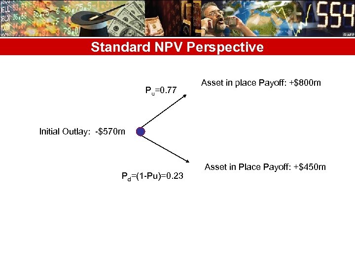Standard NPV Perspective Pu=0. 77 Asset in place Payoff: +$800 m Initial Outlay: -$570 m Pd=(1 -Pu)=0. 23 Asset in Place Payoff: +$450 m

Additional Capacity Investment • The additional capacity would require $200 m in additional investment one year from now, and is expected to increase the present value of cash flows by 30% in each scenario (i. e. , an additional $240 m for the favorable outcome, and an additional $135 m for the unfavorable outcome).

Standard NPV Perspective • Standard NPV would recognize a cash outflow of $570 m today, an outflow of $200 m one year from now, and values in one year of $1, 040 m ($800 + $240) with 77% probability, or $585 m ($450 + $135) with 23% probability.

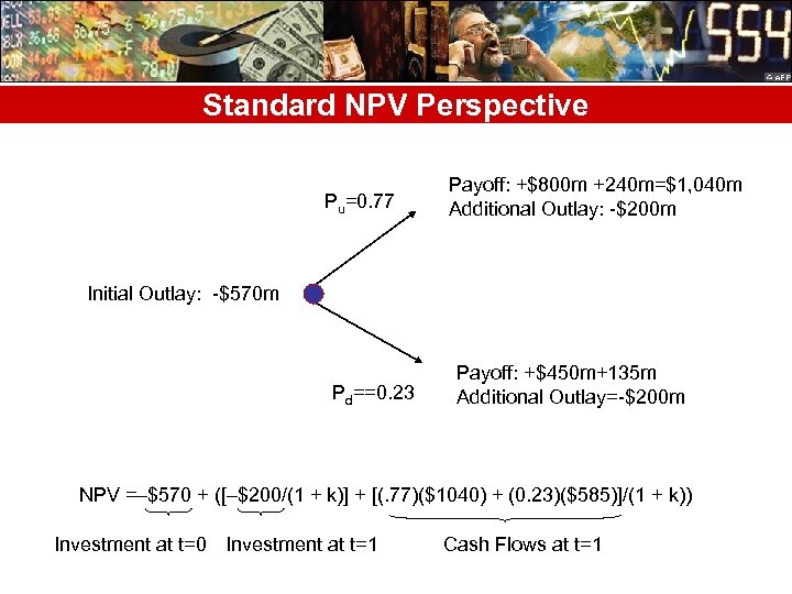Standard NPV Perspective Pu=0. 77 Payoff: +$800 m +240 m=$1, 040 m Additional Outlay: -$200 m Initial Outlay: -$570 m Pd==0. 23 Payoff: +$450 m+135 m Additional Outlay=-$200 m NPV =–$570 + ([–$200/(1 + k)] + [(. 77)($1040) + (0. 23)($585)]/(1 + k)) Investment at t=0 Investment at t=1 Cash Flows at t=1

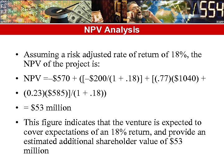NPV Analysis • Assuming a risk adjusted rate of return of 18%, the NPV of the project is: • NPV =–$570 + ([–$200/(1 +. 18)] + [(. 77)($1040) + • (0. 23)($585)]/(1 +. 18)) • = $53 million • This figure indicates that the venture is expected to cover expectations of an 18% return, and provide an estimated additional shareholder value of $53 million

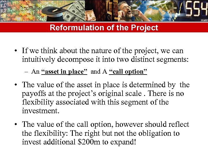Reformulation of the Project • If we think about the nature of the project, we can intuitively decompose it into two distinct segments: – An “asset in place” and A “call option” • The value of the asset in place is determined by the payoffs at the project’s original scale. There is no flexibility associated with this segment of the investment. • The value of the call option, however should reflect the flexibility: The right but not the obligation to invest additional $200 m to expand!

Failure of the Standard NPV • Standard NPV approaches properly value the asset-in place, but undervalue the option because they fail to recognize the flexibility inherent in the second segment of the project.

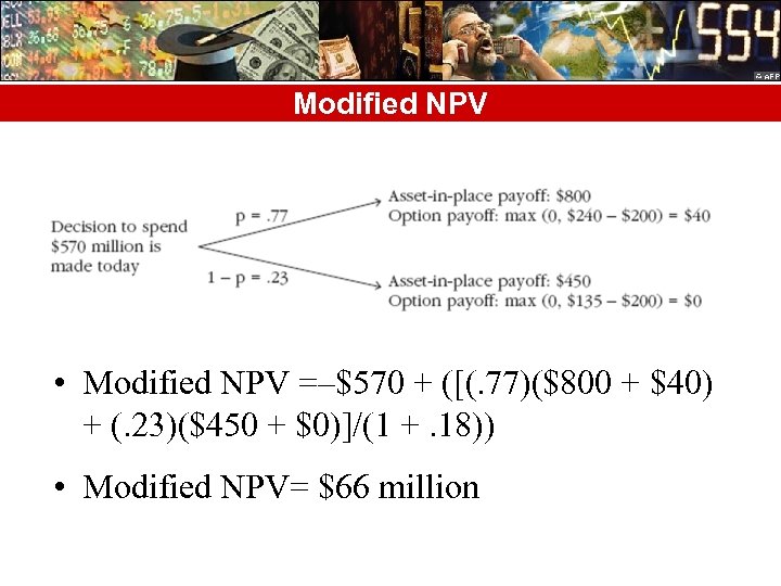Modified NPV • Modified NPV =–$570 + ([(. 77)($800 + $40) + (. 23)($450 + $0)]/(1 +. 18)) • Modified NPV= $66 million

Discussion and Summary • This result indicates that incorporating flexibility adds over 24% to the project value, and strengthens the case you will present to your venture backers. • The process used here to value this growth option can be used to evaluate other options as well, options more obscure and less restrictive than this simplified example. – For instance a staged entry into a market, where an initial commitment made today to “test the waters” may generate significant future opportunities. – Alternatively, consider a research and development program, where the results of today’s research may yield new products and cash flows never before considered.

The point is that. . • “…where managers historically have relied on instinct to build in excess capacity, test the waters, or engage in R&D, real option valuation approaches provide a systematic way to evaluate decisions to engage in these activities, and to set guidelines for how much to spend on them”.

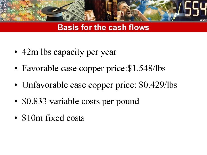
Production Option • Assume that you are extracting and refining copper ore from a mine in Australia, and the contents of the mine are almost depleted. • The remaining contents of the mine, estimated to be sufficient to produce 42 m lbs of refined copper, could be extracted in about one year, but only if you make additional investments to replace equipment.

Investment Problem • Spot prices of copper on the London Metal Exchange have been quite volatile, and are expected at year-end to be either $1. 548 per pound with a 45% probability, or $0. 429 per pound with a 55% probability. • Variable costs of refinement are expected to be $0. 833 per pound, and fixed extraction costs are estimated at $10 million for the year. • The risk-adjusted required return for the investment is 15%, and special arrangements with the Australian government allow you to realize tax-free income. • What is the most you should invest in additional equipment?

Basis for the cash flows • 42 m lbs capacity per year • Favorable case copper price: $1. 548/lbs • Unfavorable case copper price: $0. 429/lbs • $0. 833 variable costs per pound • $10 m fixed costs

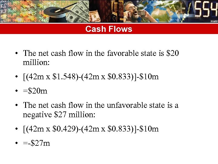Cash Flows • The net cash flow in the favorable state is $20 million: • [(42 m x $1. 548)-(42 m x $0. 833)]-$10 m • =$20 m • The net cash flow in the unfavorable state is a negative $27 million: • [(42 m x $0. 429)-(42 m x $0. 833)]-$10 m • =-$27 m

Standard NPV Approach • PV (CF) =[(. 45)($20) + (. 55)(–$27)]/(1 +. 15) • PV(CF)=–$5 million • This calculation indicates you should be unwilling to invest any further in this mine

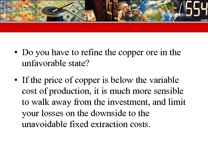• Do you have to refine the copper ore in the unfavorable state? • If the price of copper is below the variable cost of production, it is much more sensible to walk away from the investment, and limit your losses on the downside to the unavoidable fixed extraction costs.

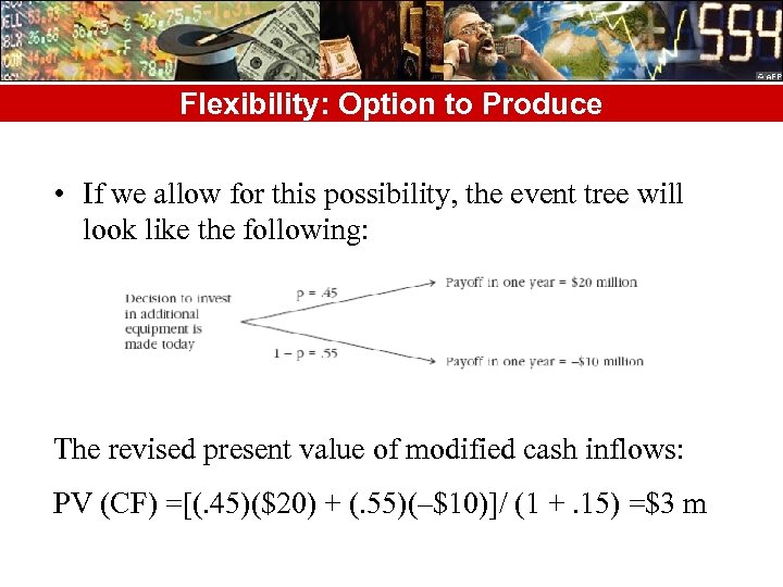Flexibility: Option to Produce • If we allow for this possibility, the event tree will look like the following: The revised present value of modified cash inflows: PV (CF) =[(. 45)($20) + (. 55)(–$10)]/ (1 +. 15) =$3 m

• In this case, the option to produce increases the value of cash inflows from the mine to $3 m and that any equipment replacement expenditures less than $3 m will create shareholder value!

Discussion and Summary • Many managers, especially in ventures dependent on natural resources, decide on a periodic basis whether or not to produce. • While this example is simplified to assume that such a decision is made once, it is straightforward to extend it to incorporate periodic production decisions. • This example shows that admitting the possibility of unfavorable outcomes may significantly change the evaluation of a project. • If operating flexibility is present, it is reasonable to incorporate it in the initial evaluation of a project’s value.

Abandonment Options: Exit Strategy • Suppose that you are a planning manager for a natural gas utility, and you are considering a proposal to develop and operate a gas main extension to serve an expanding residential community. • The value of the project is driven primarily by the price of natural gas, a highly volatile commodity. • The main extension requires $340 million to construct and will generate future cash inflows that one year from now are expected to have a present value of either $560 million or $182 million. These two outcomes are equally likely.

Traditional NPV Perspective • Assuming a 16% risk adjusted discount rate the NPV of the Project: – = –$340 + ([(. 5)($560 + (. 5)($182)]/(1 +. 16)) – = –$20 million • which indicates that the project should not be accepted!

Introducing Option to Exit • But suppose that a local distribution company (LDC) has entered into an agreement with you whereby it agrees to purchase the extension from you one year from now for $250 million, at your option. • Obviously, you would only agree to the sale in the less favorable state, and your project valuation

The Value of Exit Option • Modified NPV with the consideration of exit option: = –$340 + ([(. 5)($560) + (. 5)($250)]/(1 +. 16)) = $9 million • Incorporating the ability to sell the extension causes the project to be acceptable from a shareholder value perspective.

Discussion and Summary • It is not uncommon for the managers to admit the possibility of unfavorable outcomes before a project begins, and many implementation plans include an exit strategy. • This example demonstrates that formally incorporating an exit strategy into analyses can cause project acceptance signals to reverse. • Admitting the possibility of unfavorable outcomes has a significant impact on the project value, when there is a favorable consequence to an unfavorable outcome! In this case selling the extension has more value than holding it! • Making capital assets adaptable to other uses increases the value of exit option!!

Refinements on Method • The simple framework we introduced so far suffers from oversimplification. We have considerable challenges to improve the practicality of the real options valuation, but we can start with one: – The examples are formulated as binomial processes where two outcomes are considered at the end of the year! Can we consider more outcomes?

Binomial Process • If an uncertain variable follows a binomial process, its value will either increase by an up movement to an up state, or decrease by a down movement to a down state. • The magnitudes of the up and down movements, and their probabilities, depend upon the degree of uncertainty surrounding the movements of the variable. • While a binomial formulation is convenient for expositional purposes, two possible outcomes at the end of a year is clearly an unrealistic depiction of most processes.

Allowing more outcomes • If we take uncertainty in smaller pieces, i. e if we adjust our measure of annual uncertainty to an equivalent measure of quarterly uncertainty, and model proportionate up and down movements in the uncertain variable during each three-month period, we allow for four binomial trials within the year which results in five annual outcomes.

An Example: N=4 trials, N+1=5 Outcomes • In the following tree, PV, evolves to either PV+ or PV– at the end of three months. From each of these nodes, project value can increase or decrease once again, with the same proportional up and down movements. Note that the some nodes like PV+- can be reached in more than one set of movements. Four binomial trials within the year generates five possible outcomes at the end of the year,

From Discrete time to Continuous Time • As the length of time between binomial trials approaches zero, the result is a continuous distribution of future possible outcomes of the uncertain variable. If the uncertain variable is the price of a security underlying an option contract, the binomial model converges to the Black-Scholes option pricing model.

Black-Scholes Option Pricing Model • The Black-Scholes model solves for option values as a function of five variables: – exercise price, – time to expiration, – discount rate, – the present value of the underlying asset, – volatility.

Mapping B-S variables with Real Options • The exercise price: – For a capital investment project, this is the dollar value in the future (not discounted to the present) of the capital expenditures necessary to implement the flexible portion of the project. – For example, this is the cost of the plant and equipment necessary to support full scale production ($12 million) in the pharmaceutical example (the timing option)

Mapping B-S variables with Real Options • The Time to Expiration: – The length of time before a decision must be made and capital committed. In all of our examples, this was one year.

Mapping B-S variables with Real Options • The Discount Rate: – The discount rate, which is used to convert future amounts to present values.

Mapping B-S variables with Real Options • The Value of the Underlying Asset: – For an option written on a share of stock, this is the current value of the share of stock; for a capital investment project, this is the present value of the cash inflows expected from the flexible portion of the project. – For example, in the growth option (e-commerce) example, this would be the probability weighted average of $240 million and $135 million, discounted back to the present.

Mapping B-S variables with Real Options • Volatility: – Volatility, is measured as the standard deviation (sigma) of the rate of growth in the value of the underlying asset.

Application B-S Model to the Timing Option • Here the exercise price is the $12 million investment to construct the plant one year from now. • Time to expiration is 365 days (one year), • The discount rate (for simplicity) is 20% • Volatility: We haven’t used a sigma in our calculations, a sigma of 1. 1, or 110%, was used to determine the range of outcomes ($39 million to $4. 3 million) and their probabilities. • Value of the Underlying Asset: PV =[(. 33)($39. 00) + (. 67)($4. 30)]/(1 +. 2) • =13. 13 million

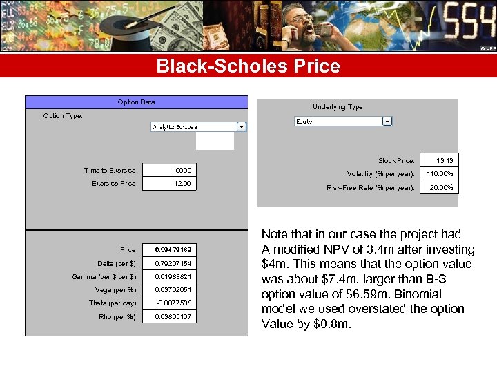Black-Scholes Price Option Data Option Type: Underlying Type: Stock Price: 13. 13 Volatility (% per year): 110. 00% Risk-Free Rate (% per year): 20. 00% Time to Exercise: 1. 0000 Exercise Price: 12. 00 Price: 6. 59479189 Delta (per $): 0. 79207154 Gamma (per $): 0. 01983821 Vega (per %): 0. 03762051 Theta (per day): -0. 0077538 Rho (per %): 0. 03805107 Note that in our case the project had A modified NPV of 3. 4 m after investing $4 m. This means that the option value was about $7. 4 m, larger than B-S option value of $6. 59 m. Binomial model we used overstated the option Value by $0. 8 m.

Challenge in using B-S Model to value Real Options • Black-Scholes model assumes that the expected value of the underlying asset grows over time at the risk-adjusted discount rate, and that the risk of the underlying asset is constant over time. • Black-Scholes model works best if there is only one decision to be made on some future date, while the binomial model applies if there is a series of sequential decisions or multiple options.

Challenge… • The biggest difficulty is that many projects with option elements also include one or more assets-in-place. • For instance in the growth option example the cash flows in the first year are not subject to any flexibility, and are properly valued with standard discounted cash flow techniques. • Black-Scholes valuation requires the identification of assetsin-place where they are present, and the separation of assets -in-place from option elements for purposes of defining Black- Scholes inputs. • This requires careful strategic framing of the project, and takes a little practice.

Binomial Movements • Starting Value (asset price at t=0)=S 0=13 • u=eσ=3 for σ=110% or 1. 1 • d=1/eσ =0. 33 for σ=110% or 1. 1 • Su=S 0 u=13 x 3=39 • Sd=S 0 d=13 x 0. 33=4. 3

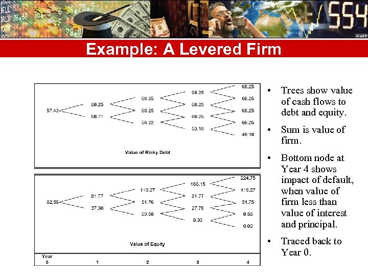Example: A Levered Firm • Trees show value of cash flows to debt and equity. • Sum is value of firm. • Bottom node at Year 4 shows impact of default, when value of firm less than value of interest and principal. • Traced back to Year 0.

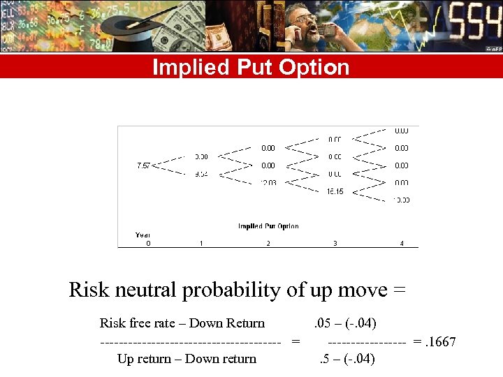Implied Put Option Risk neutral probability of up move = Risk free rate – Down Return. 05 – (-. 04) -------------------- =. 1667 Up return – Down return. 5 – (-. 04)

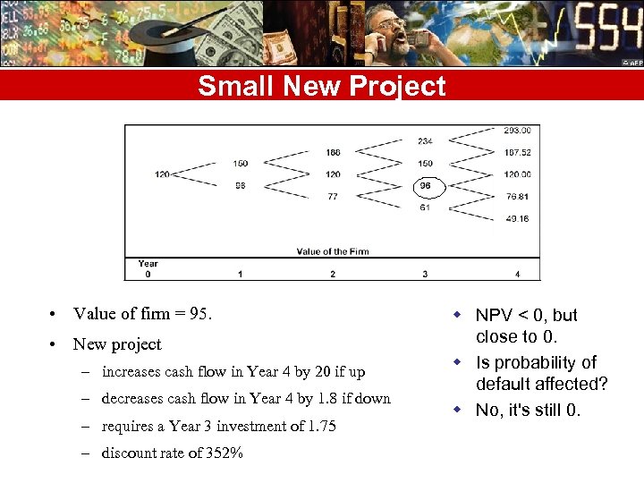Small New Project • Value of firm = 95. • New project – increases cash flow in Year 4 by 20 if up – decreases cash flow in Year 4 by 1. 8 if down – requires a Year 3 investment of 1. 75 – discount rate of 352% w NPV < 0, but close to 0. w Is probability of default affected? w No, it's still 0.

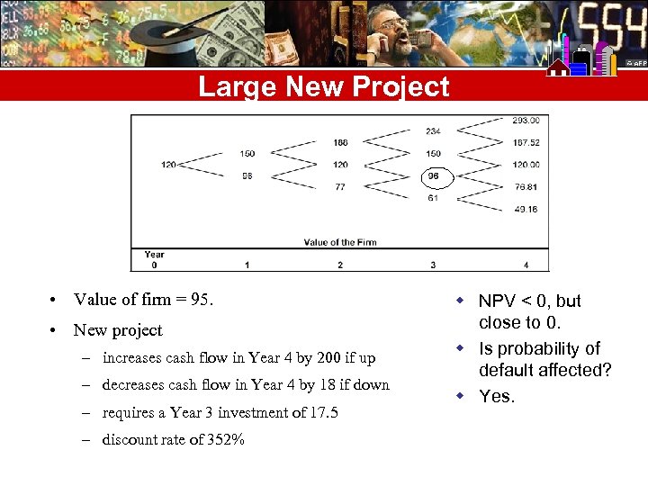Large New Project • Value of firm = 95. • New project – increases cash flow in Year 4 by 200 if up – decreases cash flow in Year 4 by 18 if down – requires a Year 3 investment of 17. 5 – discount rate of 352% w NPV < 0, but close to 0. w Is probability of default affected? w Yes.

Asset Substitution • If larger new project adopted, and down move occurs at Year 4, firm's value declines $9. 45 million below debt obligation. • Implied put option increases by $9. 45 at Year 4. • Value of put option at Year 3 is 7. 5 = 0. 833 x 9. 45 / 1. 05 where 0. 833 = 1 – 0. 1667. • Managers increase shareholder value, decrease value of debt, by adopting new larger project.

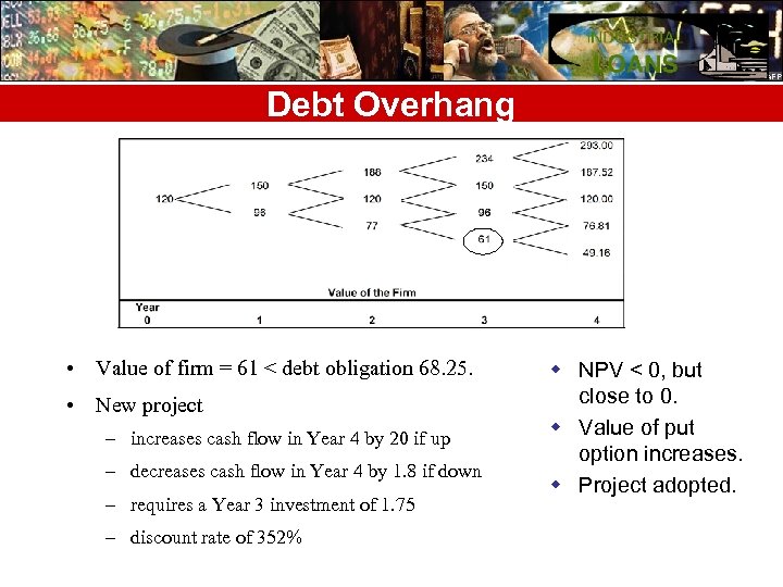Debt Overhang • Value of firm = 61 < debt obligation 68. 25. • New project – increases cash flow in Year 4 by 20 if up – decreases cash flow in Year 4 by 1. 8 if down – requires a Year 3 investment of 1. 75 – discount rate of 352% w NPV < 0, but close to 0. w Value of put option increases. w Project adopted.

Capital Structure • Debtholders anticipate possibility of asset substitution and debt overhang. • They respond by increasing the cost of debt. • Firms' managers choose to hold less debt than is optimal. • Value of firms' equity less as a result, due to foregone tax shields.

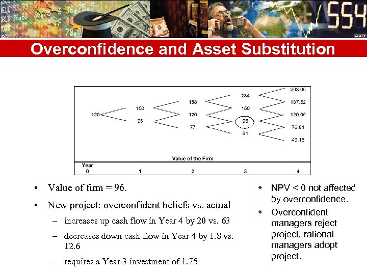Overconfidence and Asset Substitution • Value of firm = 96. • New project: overconfident beliefs vs. actual – increases up cash flow in Year 4 by 20 vs. 63 – decreases down cash flow in Year 4 by 1. 8 vs. 12. 6 – requires a Year 3 investment of 1. 75 w NPV < 0 not affected by overconfidence. w Overconfident managers reject project, rational managers adopt project.

Biased Backdrop • Excessive optimism and overconfidence induce managers to – overestimate project NPV – overestimate tax shield benefits from debt – underestimate the costs associated with financial distress • These biases increase the tendency to be overleveraged. • Agency conflicts operate in the other direction.

Behavioral Biases Counter Agency Conflicts • Once a debt contract is in place, investment policy can impact the value of the implicit put. • Shareholders and debtholders share the value of a positive NPV project, but the shares need not be positive amounts. • Agency conflicts increase the cost of debt. • Mild excessive optimism and overconfidence induce managers to behave more favorably towards debtholders, thereby leading to increased leverage.