Rational Shapes of the Volatility Surface Jim Gatheral

Rational Shapes of the Volatility Surface Jim Gatheral Global Equity-Linked Products Merrill Lynch Risk 2000, Tuesday 13 June 2000

References • Bakshi, G. , Cao C. , Chen Z. , “Empirical Performance of Alternative Option Pricing Models” Journal of Finance, 52, 2003 -2049. • J. Gatheral, Courant Institute of Mathematical Sciences Lecture Notes, http: //www. math. nyu. edu/fellows_fin_math/gatheral/. • Hardy M. Hodges. “Arbitrage Bounds on the Implied Volatility Strike and Term Structures of European-Style Options. ” The Journal of Derivatives, Summer 1996. • Roger Lee, “Local volatilities in Stochastic Volatility Models”, Working Paper, Stanford University, 1999. • R. Merton, “Option Pricing When Underlying Stock Returns are Discontinuous, ” Journal of Financial Economics, 3, January-February 1976. Risk 2000, Tuesday 13 June 2000 2

Goals • Derive arbitrage bounds on the slope and curvature of volatility skews. • Investigate the strike and time behavior of these bounds. • Specialize to stochastic volatility and jumps. • Draw implications for parameterization of the volatility surface. Risk 2000, Tuesday 13 June 2000 3

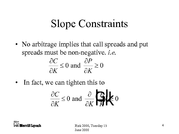Slope Constraints • No arbitrage implies that call spreads and put spreads must be non-negative. i. e. • In fact, we can tighten this to Risk 2000, Tuesday 13 June 2000 4

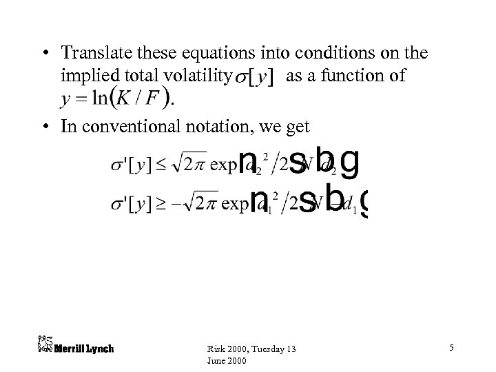• Translate these equations into conditions on the implied total volatility as a function of. • In conventional notation, we get Risk 2000, Tuesday 13 June 2000 5

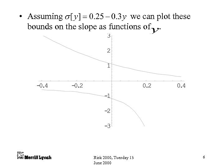• Assuming we can plot these bounds on the slope as functions of. Risk 2000, Tuesday 13 June 2000 6

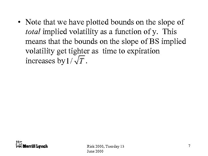• Note that we have plotted bounds on the slope of total implied volatility as a function of y. This means that the bounds on the slope of BS implied volatility get tighter as time to expiration increases by. Risk 2000, Tuesday 13 June 2000 7

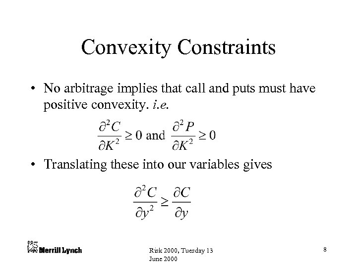Convexity Constraints • No arbitrage implies that call and puts must have positive convexity. i. e. • Translating these into our variables gives Risk 2000, Tuesday 13 June 2000 8

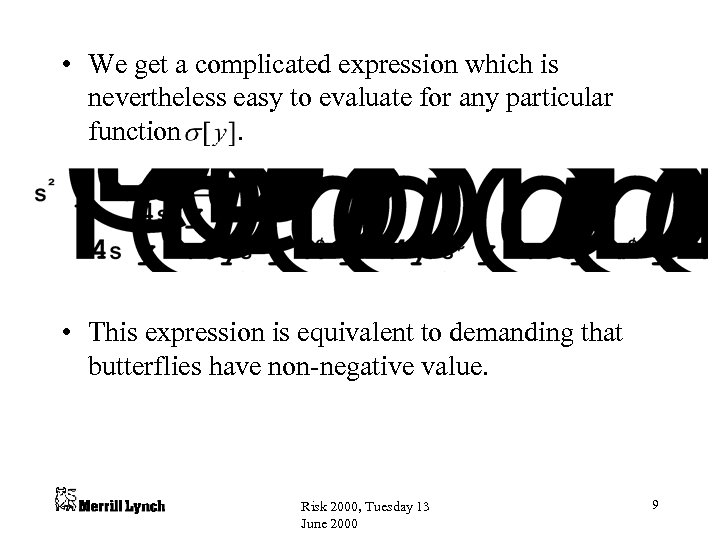• We get a complicated expression which is nevertheless easy to evaluate for any particular function. • This expression is equivalent to demanding that butterflies have non-negative value. Risk 2000, Tuesday 13 June 2000 9

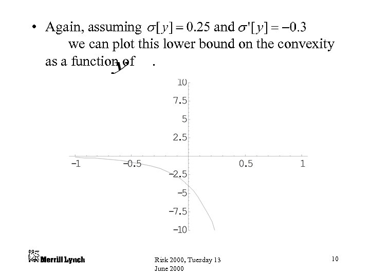• Again, assuming and we can plot this lower bound on the convexity as a function of. Risk 2000, Tuesday 13 June 2000 10

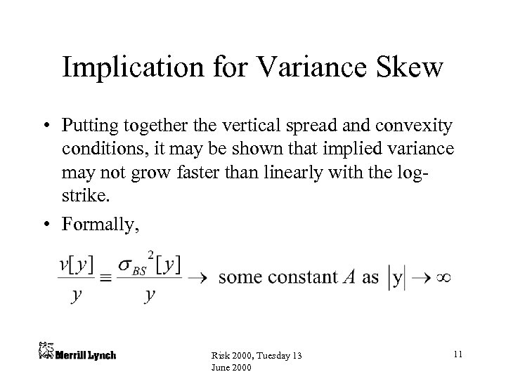Implication for Variance Skew • Putting together the vertical spread and convexity conditions, it may be shown that implied variance may not grow faster than linearly with the logstrike. • Formally, Risk 2000, Tuesday 13 June 2000 11

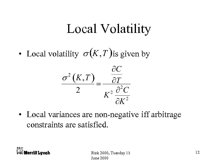Local Volatility • Local volatility is given by • Local variances are non-negative iff arbitrage constraints are satisfied. Risk 2000, Tuesday 13 June 2000 12

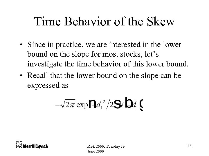Time Behavior of the Skew • Since in practice, we are interested in the lower bound on the slope for most stocks, let’s investigate the time behavior of this lower bound. • Recall that the lower bound on the slope can be expressed as Risk 2000, Tuesday 13 June 2000 13

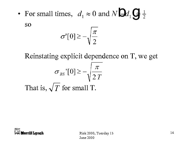• For small times, so Reinstating explicit dependence on T, we get That is, for small T. Risk 2000, Tuesday 13 June 2000 14

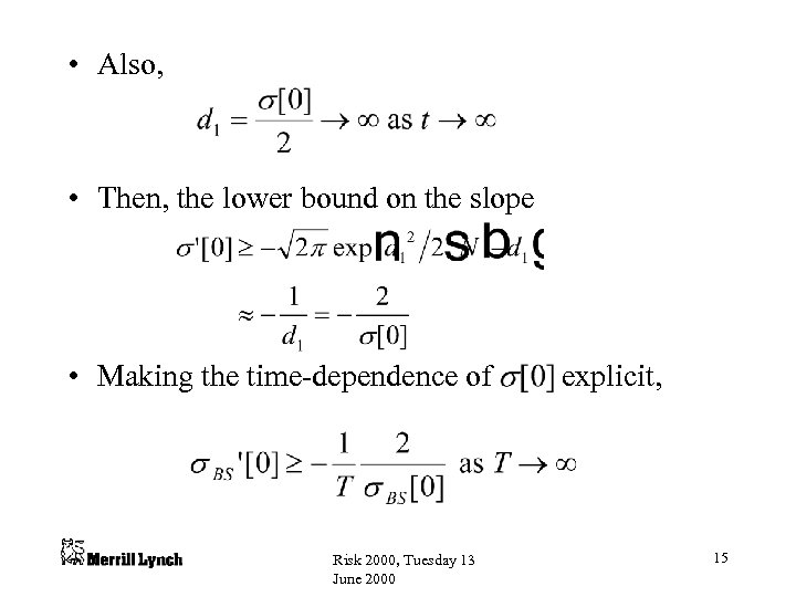• Also, • Then, the lower bound on the slope • Making the time-dependence of Risk 2000, Tuesday 13 June 2000 explicit, 15

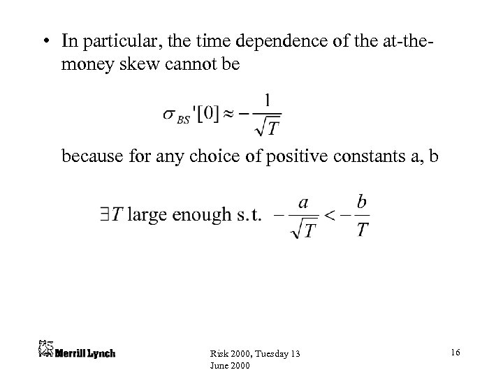• In particular, the time dependence of the at-themoney skew cannot be because for any choice of positive constants a, b Risk 2000, Tuesday 13 June 2000 16

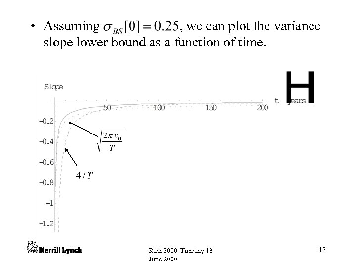• Assuming , we can plot the variance slope lower bound as a function of time. Risk 2000, Tuesday 13 June 2000 17

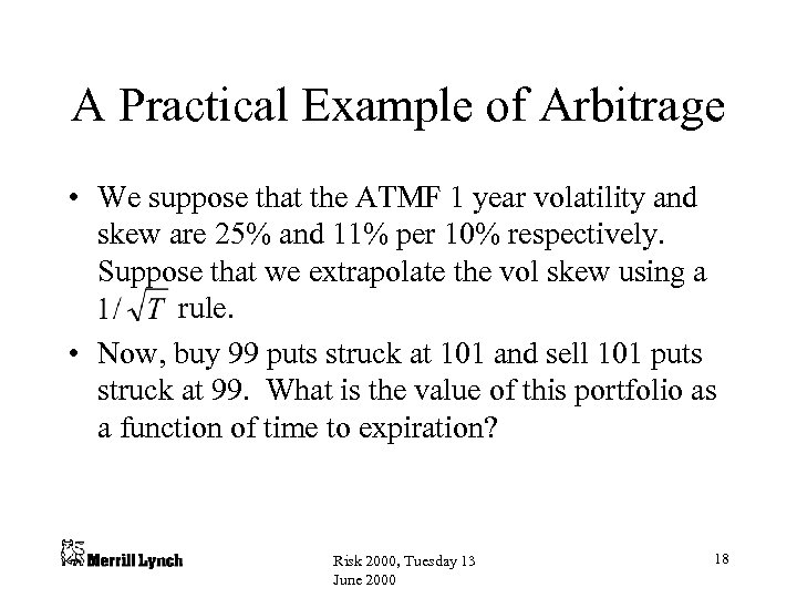A Practical Example of Arbitrage • We suppose that the ATMF 1 year volatility and skew are 25% and 11% per 10% respectively. Suppose that we extrapolate the vol skew using a rule. • Now, buy 99 puts struck at 101 and sell 101 puts struck at 99. What is the value of this portfolio as a function of time to expiration? Risk 2000, Tuesday 13 June 2000 18

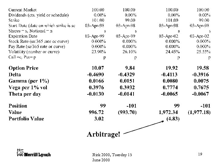Arbitrage! Risk 2000, Tuesday 13 June 2000 19

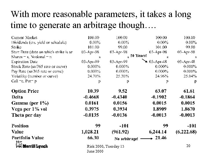With more reasonable parameters, it takes a long time to generate an arbitrage though…. 50 Years! No arbitrage! Risk 2000, Tuesday 13 June 2000 20

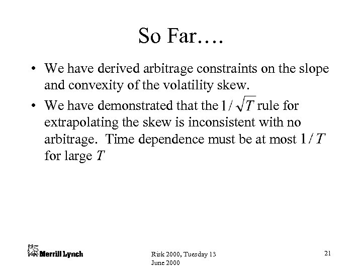So Far…. • We have derived arbitrage constraints on the slope and convexity of the volatility skew. • We have demonstrated that the rule for extrapolating the skew is inconsistent with no arbitrage. Time dependence must be at most for large T Risk 2000, Tuesday 13 June 2000 21

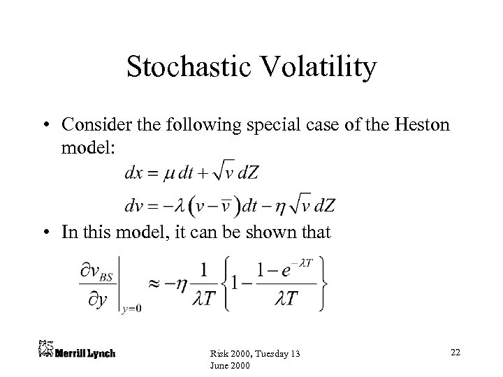Stochastic Volatility • Consider the following special case of the Heston model: • In this model, it can be shown that Risk 2000, Tuesday 13 June 2000 22

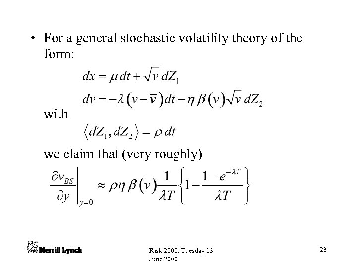• For a general stochastic volatility theory of the form: with we claim that (very roughly) Risk 2000, Tuesday 13 June 2000 23

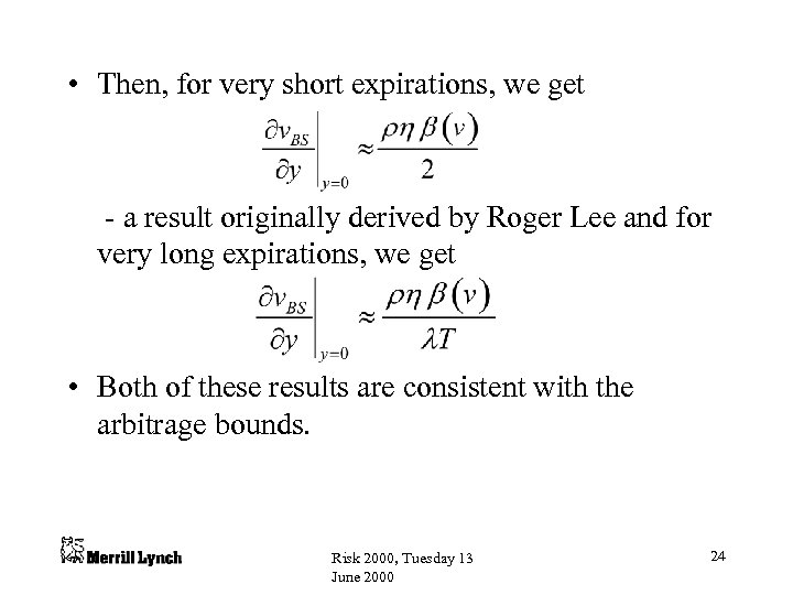• Then, for very short expirations, we get - a result originally derived by Roger Lee and for very long expirations, we get • Both of these results are consistent with the arbitrage bounds. Risk 2000, Tuesday 13 June 2000 24

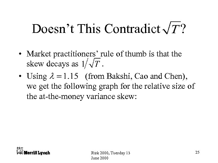Doesn’t This Contradict ? • Market practitioners’ rule of thumb is that the skew decays as. • Using (from Bakshi, Cao and Chen), we get the following graph for the relative size of the at-the-money variance skew: Risk 2000, Tuesday 13 June 2000 25

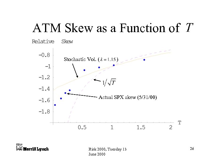ATM Skew as a Function of Stochastic Vol. ( ) Actual SPX skew (5/31/00) Risk 2000, Tuesday 13 June 2000 26

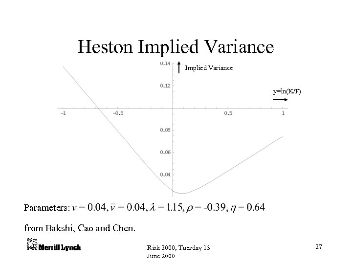Heston Implied Variance y=ln(K/F) Parameters: from Bakshi, Cao and Chen. Risk 2000, Tuesday 13 June 2000 27

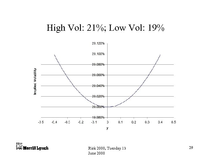
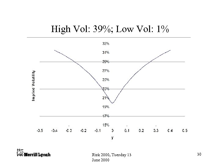
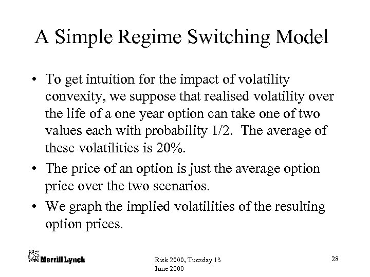A Simple Regime Switching Model • To get intuition for the impact of volatility convexity, we suppose that realised volatility over the life of a one year option can take one of two values each with probability 1/2. The average of these volatilities is 20%. • The price of an option is just the average option price over the two scenarios. • We graph the implied volatilities of the resulting option prices. Risk 2000, Tuesday 13 June 2000 28

High Vol: 21%; Low Vol: 19% Risk 2000, Tuesday 13 June 2000 29

High Vol: 39%; Low Vol: 1% Risk 2000, Tuesday 13 June 2000 30

Intuition • As , implied volatility tends to the highest volatility. • If volatility is unbounded, implied volatility must also be unbounded. • From a trader’s perspective, the more out-of-themoney (OTM) an option is, the more vol convexity it has. Provided volatility is unbounded, more OTM options must command higher implied volatility. Risk 2000, Tuesday 13 June 2000 31

Asymmetric Variance Gamma Implied Variance y=ln(K/F) Parameters: Risk 2000, Tuesday 13 June 2000 32

Jump Diffusion • Consider the simplest form of Merton’s jumpdiffusion model with a constant probability of a jump to ruin. • Call options are valued in this model using the Black-Scholes formula with a shifted forward price. • We graph 1 year implied variance as a function of log-strike with : Risk 2000, Tuesday 13 June 2000 33

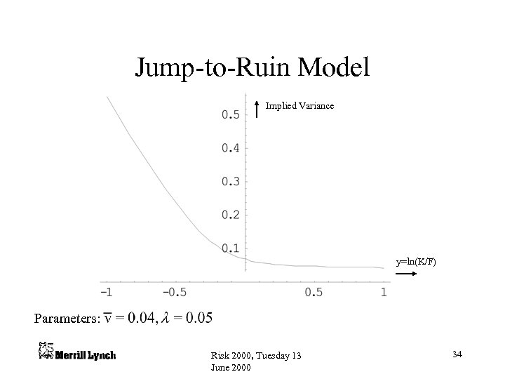Jump-to-Ruin Model Implied Variance y=ln(K/F) Parameters: Risk 2000, Tuesday 13 June 2000 34

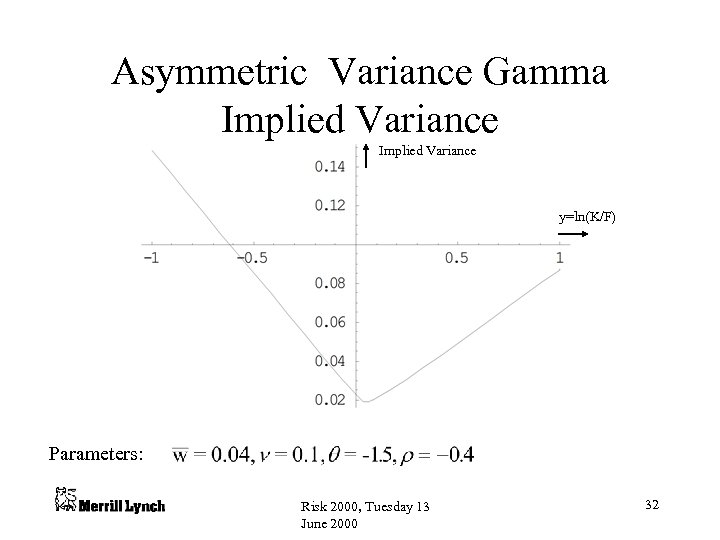
• So, even in jump-diffusion, is linear in as. • In fact, we can show that for many economically reasonable stochastic-volatility-plus-jump models, implied BS variance must be asymptotically linear in the log-strike as. • This means that it does not make sense to plot implied BS variance against delta. As an example, consider the following graph of vs. d in the Heston model: Risk 2000, Tuesday 13 June 2000 35

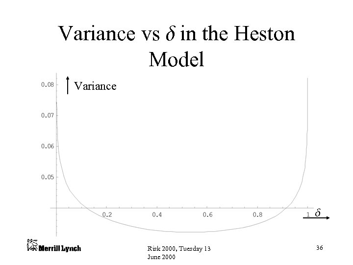Variance vs d in the Heston Model Variance d Risk 2000, Tuesday 13 June 2000 36

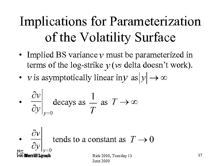Implications for Parameterization of the Volatility Surface • Implied BS variance must be parameterized in terms of the log-strike (vs delta doesn’t work). • is asymptotically linear in as • decays as • tends to a constant as as Risk 2000, Tuesday 13 June 2000 37