a74cfd1df2805e38d83fd202f5a9d975.ppt
- Количество слайдов: 119



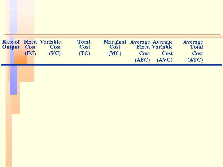
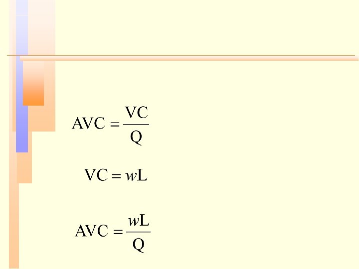
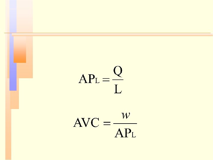
Rate of Fixed Variable Output Cost (FC) (VC) Total Cost (TC) Marginal Average Cost Fixed Variable (MC) Cost (AFC) (AVC) Average Total Cost (ATC)
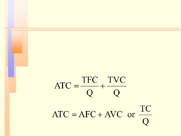


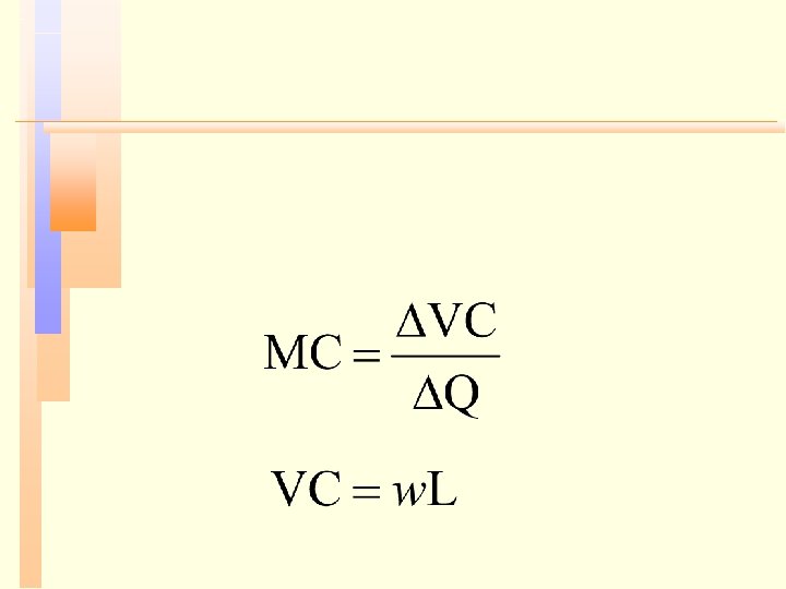
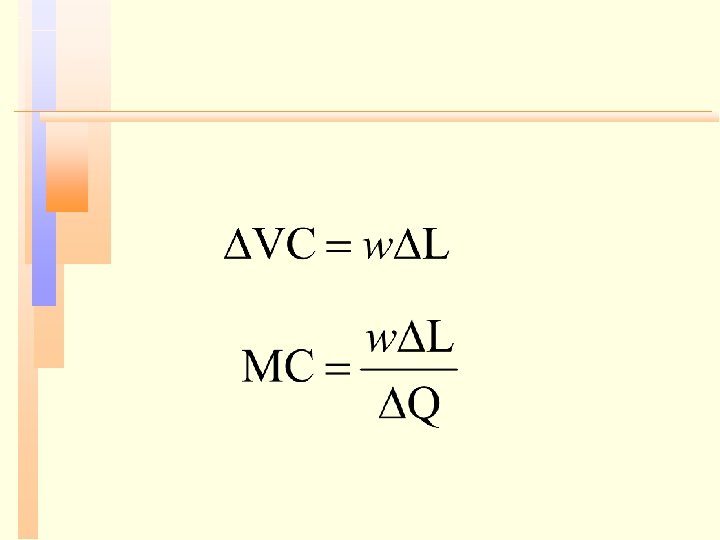
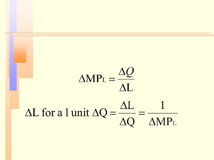
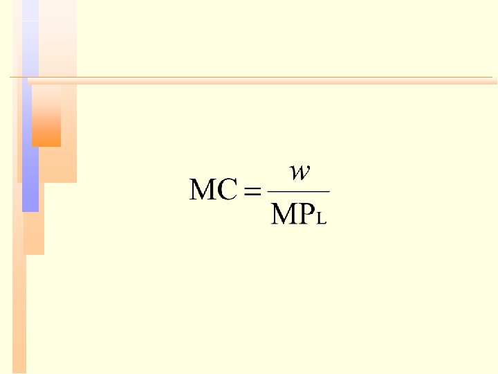


Rate of Fixed Variable Output Cost (FC) (VC) Total Cost (TC) Marginal Average Cost Fixed Variable (MC) Cost (AFC) (AVC) Average Total Cost (ATC)


Output (units per year)
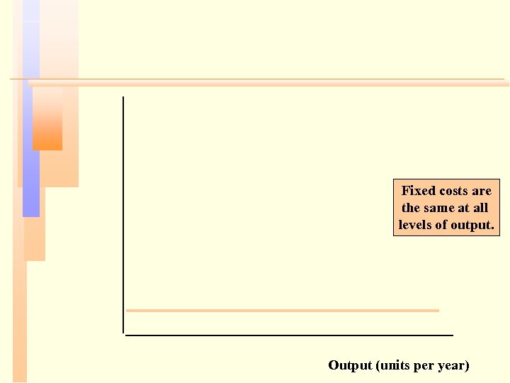
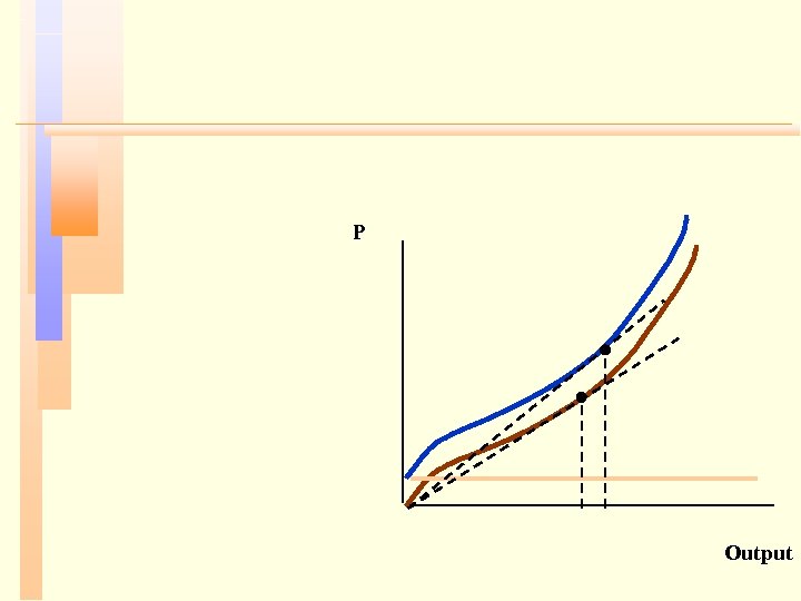
Fixed costs are the same at all levels of output. Output (units per year)
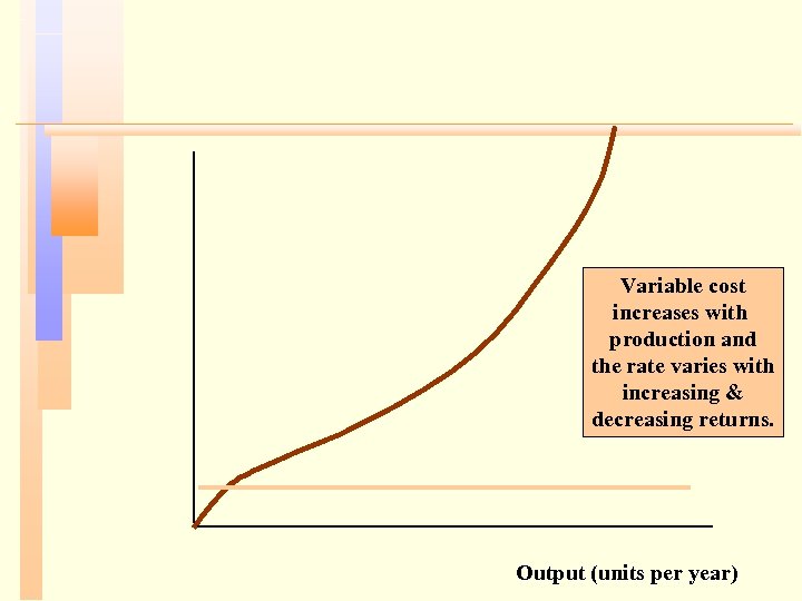
Variable cost increases with production and the rate varies with increasing & decreasing returns. Output (units per year)
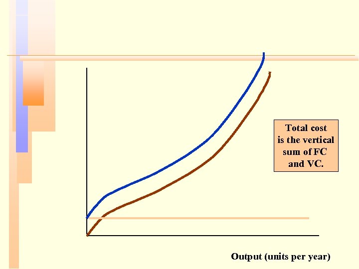
Total cost is the vertical sum of FC and VC. Output (units per year)
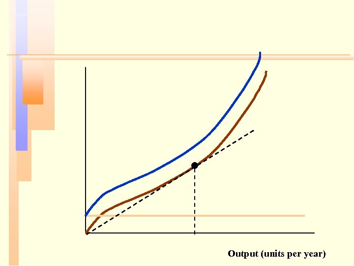
Output (units per year)
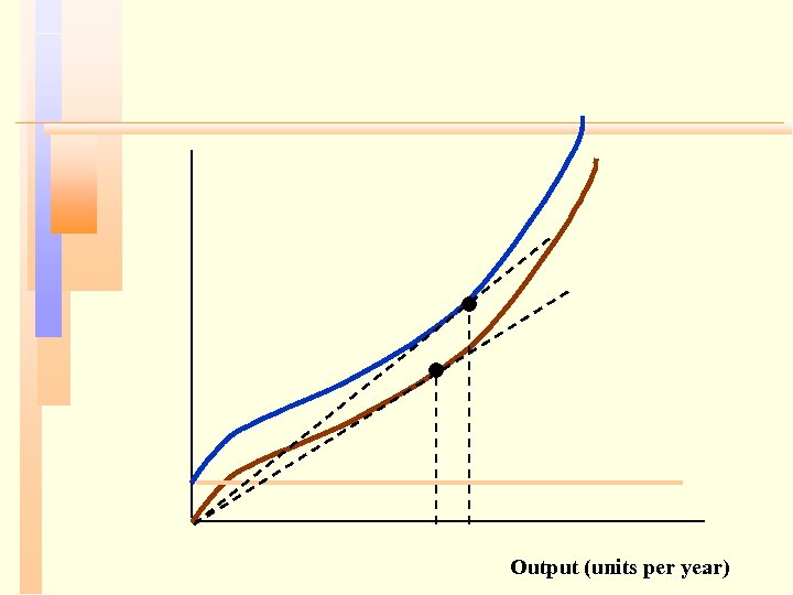
Output (units per year)
Output (units per year)
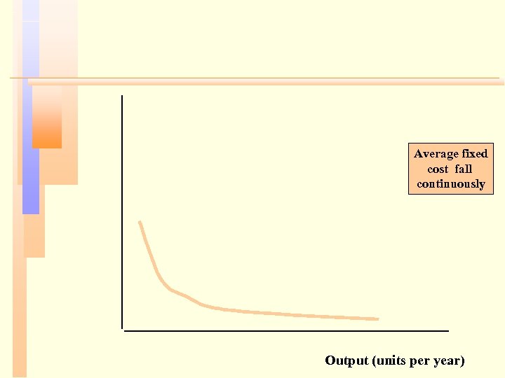
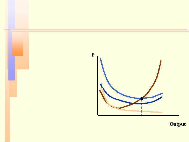
Average fixed cost fall continuously Output (units per year)
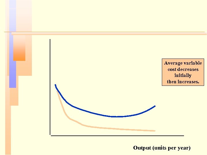
Average variable cost decreases initially then increases. Output (units per year)
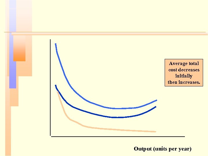
Average total cost decreases initially then increases. Output (units per year)
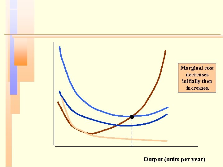
Marginal cost decreases initially then increases. Output (units per year)
P Output

P Output
P Output
P Output


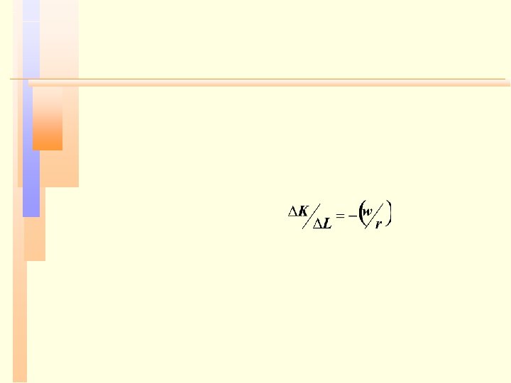

Capital per year Labor per year
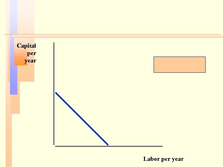
Capital per year Labor per year
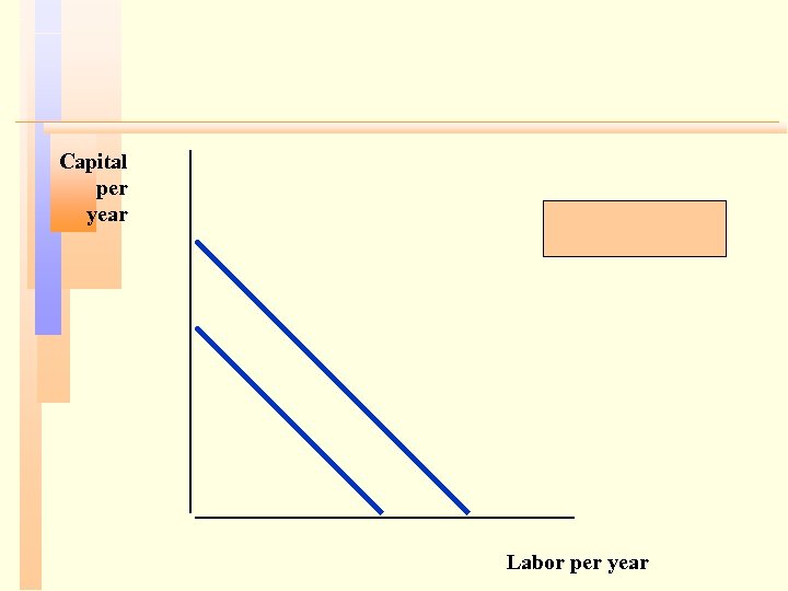
Capital per year Labor per year
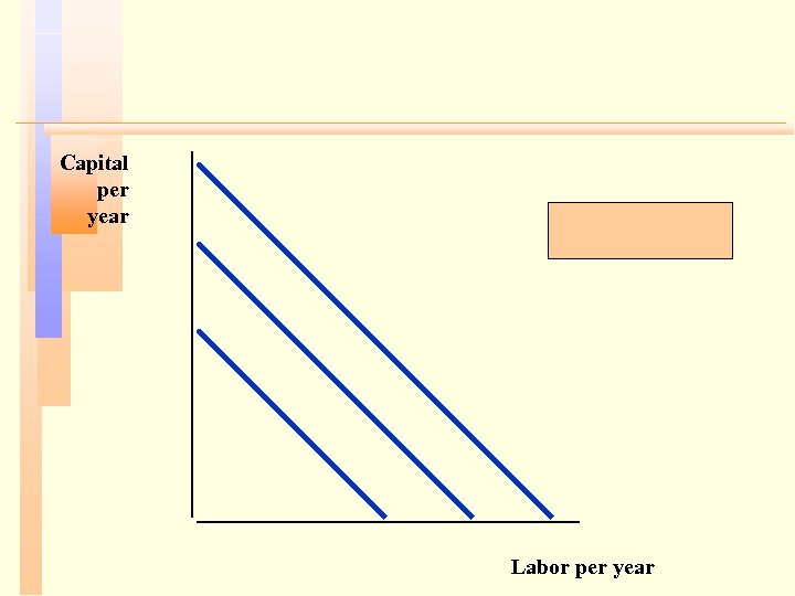
Capital per year Labor per year
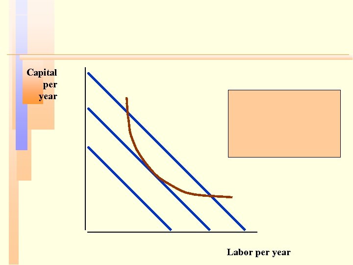
Capital per year Labor per year
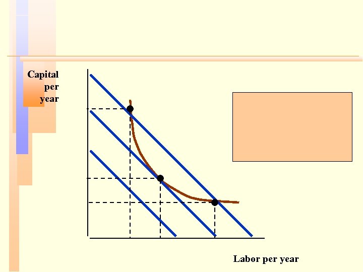
Capital per year Labor per year
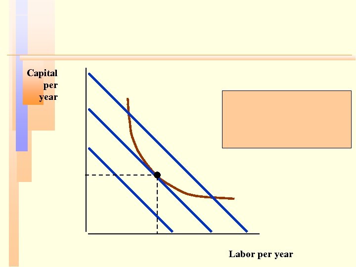
Capital per year Labor per year
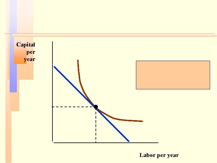
Capital per year Labor per year
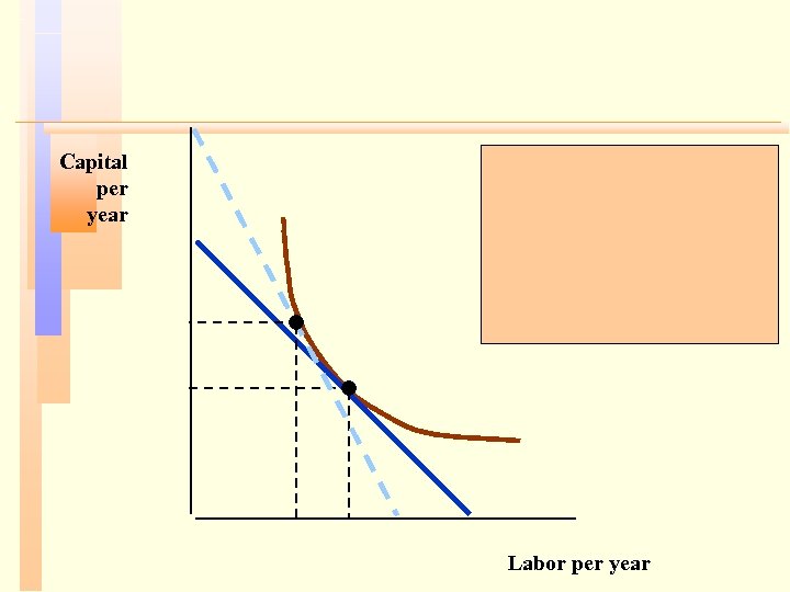
Capital per year Labor per year
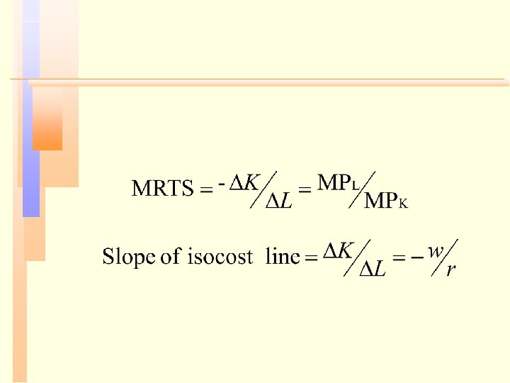
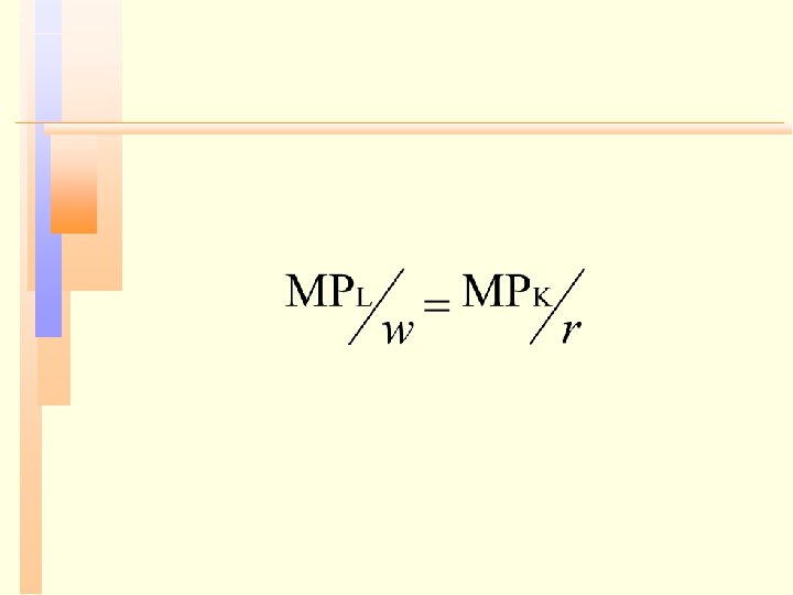


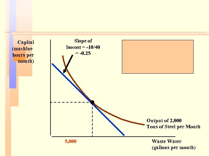
Capital (machine hours per month) Slope of isocost = -10/40 = -0. 25 Output of 2, 000 Tons of Steel per Month 5, 000 Waste Water (gallons per month)
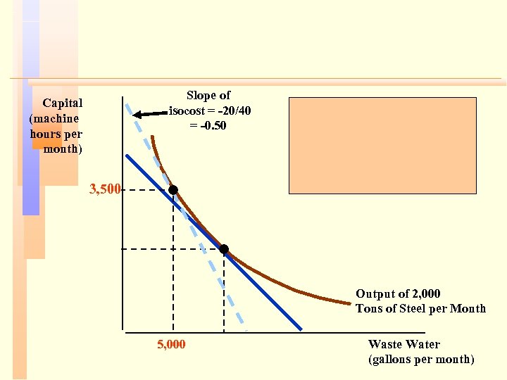
Slope of isocost = -20/40 = -0. 50 Capital (machine hours per month) 3, 500 Output of 2, 000 Tons of Steel per Month 5, 000 Waste Water (gallons per month)


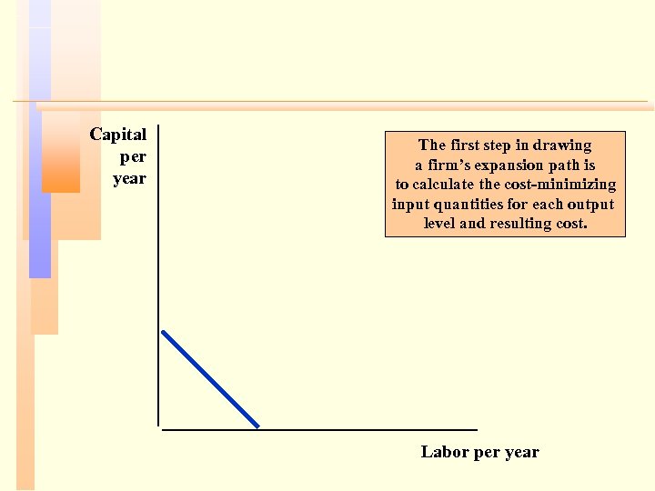
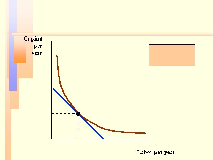
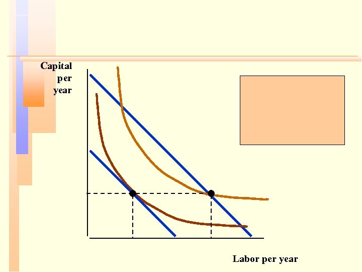
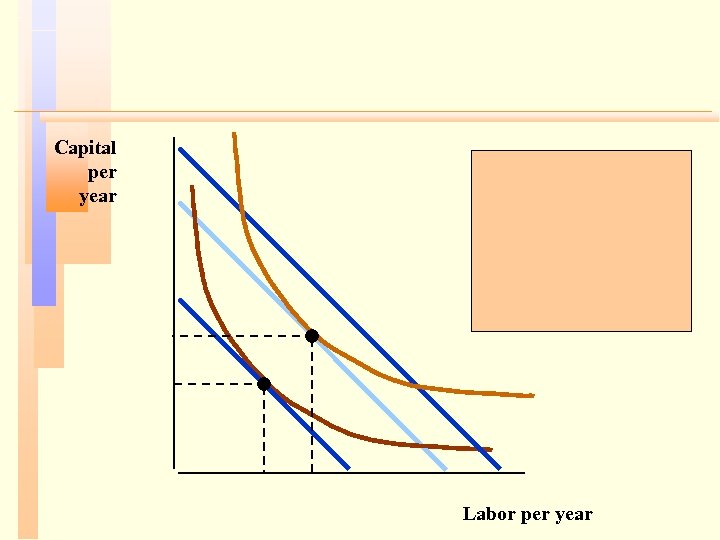
Capital per year The first step in drawing a firm’s expansion path is to calculate the cost-minimizing input quantities for each output level and resulting cost. Labor per year
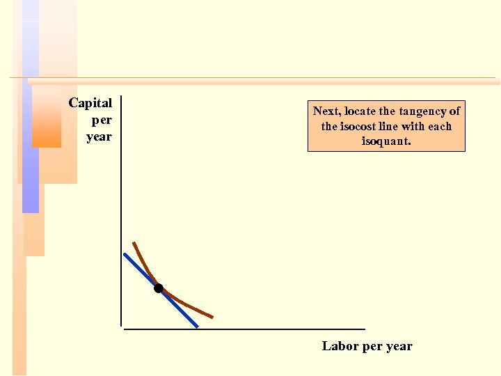
Capital per year Next, locate the tangency of the isocost line with each isoquant. Labor per year
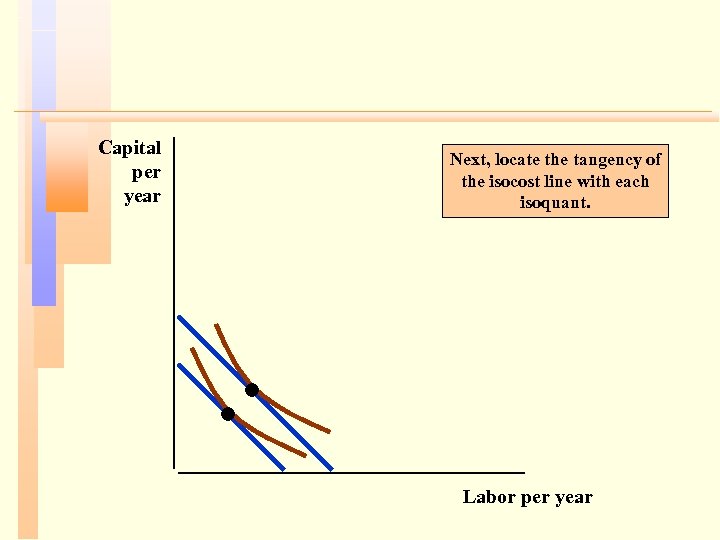
Capital per year Next, locate the tangency of the isocost line with each isoquant. Labor per year
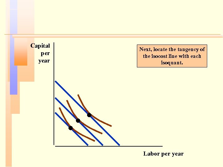
Capital per year Next, locate the tangency of the isocost line with each isoquant. Labor per year
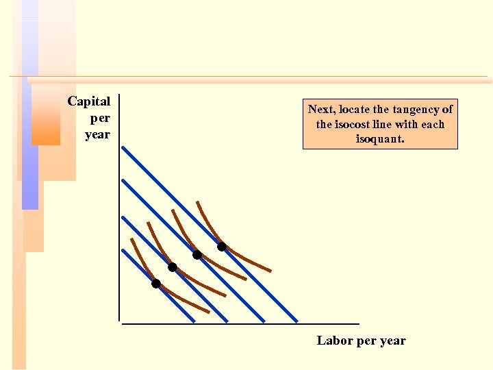
Capital per year Next, locate the tangency of the isocost line with each isoquant. Labor per year
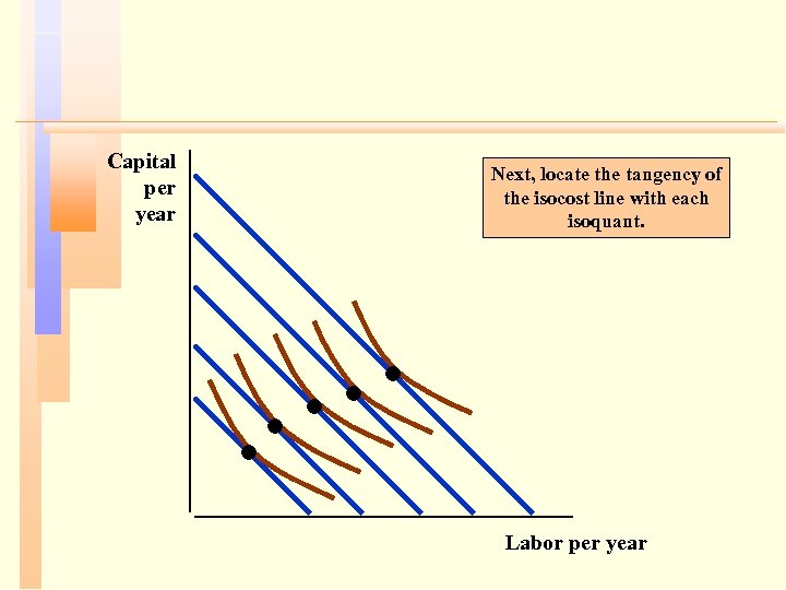
Capital per year Next, locate the tangency of the isocost line with each isoquant. Labor per year
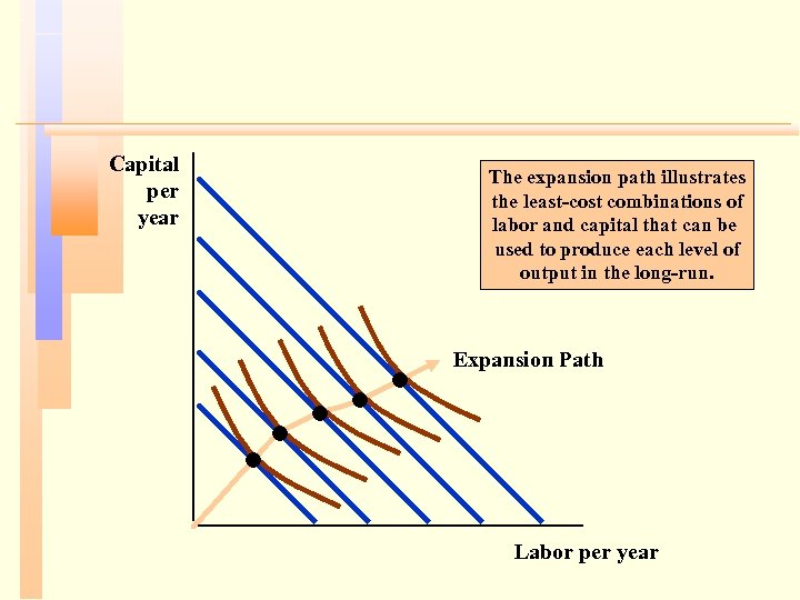
Capital per year The expansion path illustrates the least-cost combinations of labor and capital that can be used to produce each level of output in the long-run. Expansion Path Labor per year

Capital per year Labor per year
Capital per year Labor per year
Capital per year Labor per year
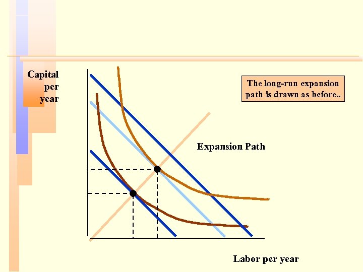
Capital per year The long-run expansion path is drawn as before. . Expansion Path Labor per year


Cost ($ per unit of output Output
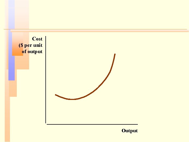
Cost ($ per unit of output Output
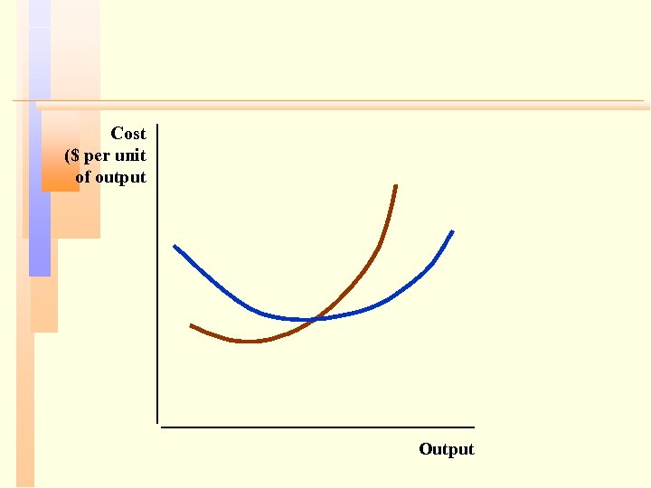
Cost ($ per unit of output Output


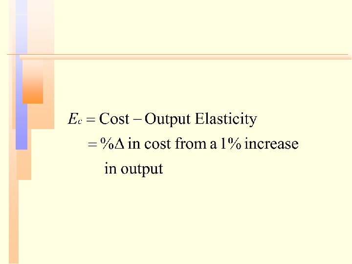
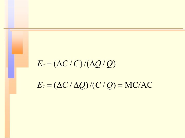


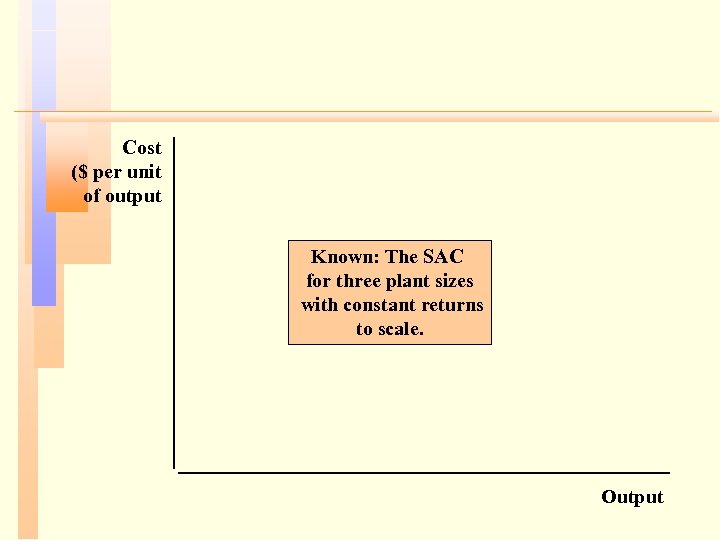
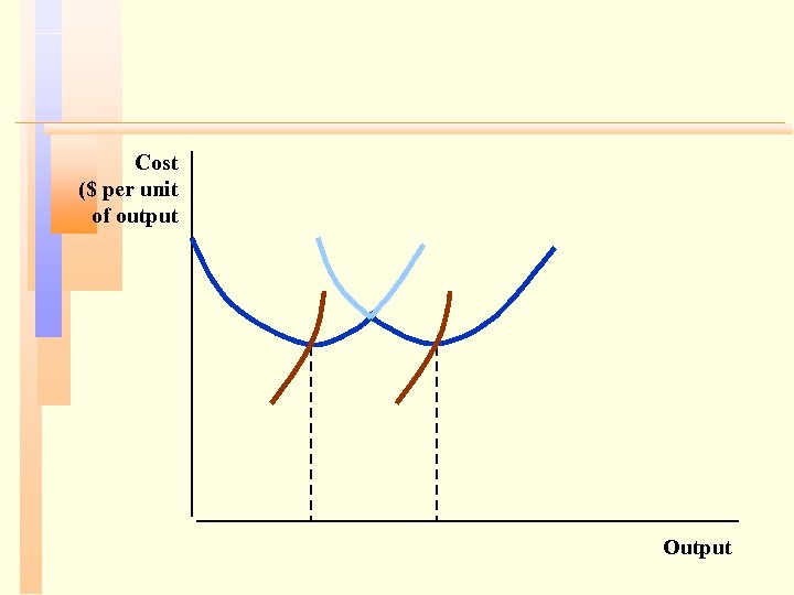
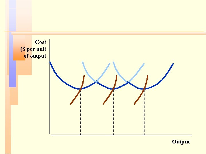
Cost ($ per unit of output Known: The SAC for three plant sizes with constant returns to scale. Output
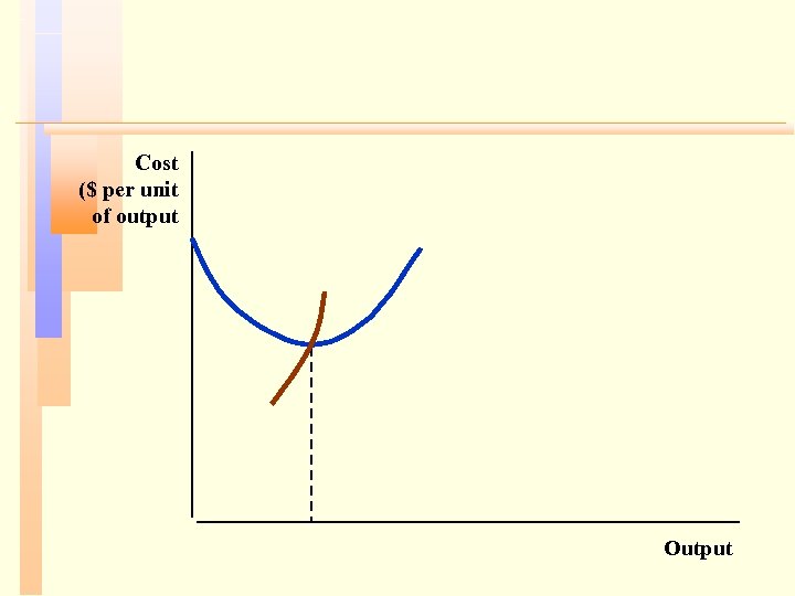
Cost ($ per unit of output Output
Cost ($ per unit of output Output
Cost ($ per unit of output Output
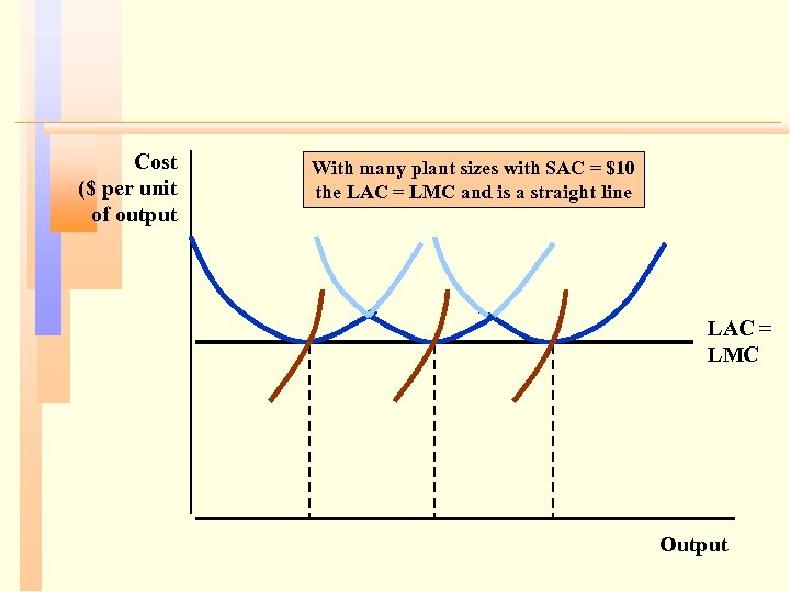
Cost ($ per unit of output With many plant sizes with SAC = $10 the LAC = LMC and is a straight line LAC = LMC Output
Cost ($ per unit of output Known: Three plant sizes with economies and diseconomies of scale. Output
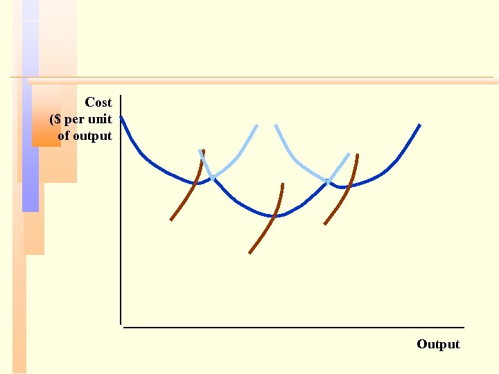
Cost ($ per unit of output Output
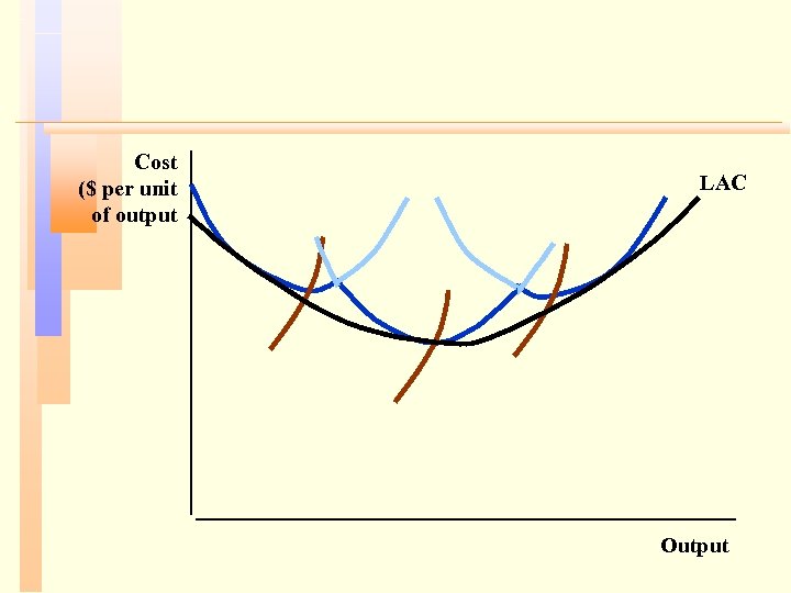
Cost ($ per unit of output LAC Output
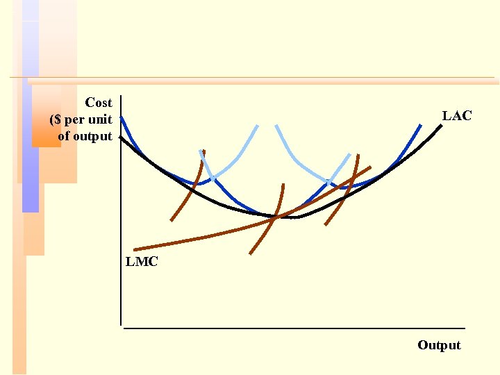
Cost ($ per unit of output LAC LMC Output
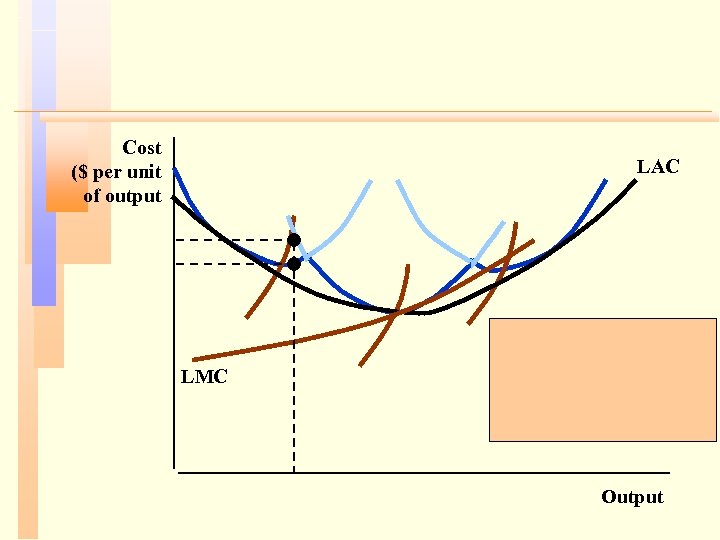
Cost ($ per unit of output LAC LMC Output


Number of tractors Number of cars
Number of tractors Number of cars
Number of tractors Number of cars




a74cfd1df2805e38d83fd202f5a9d975.ppt