R-programming http www r-project org http cran r-project

R-programming http: //www. r-project. org/ http: //cran. r-project. org/ Hung Chen

Outline • Introduction: – Historical development – S, Splus – Capability – Statistical Analysis • References • Calculator • Data Type • Resources • Simulation and Statistical Tables – Probability distributions • Programming – Grouping, loops and conditional execution – Function • Reading and writing data from files • Modeling – Regression – ANOVA • Data Analysis on Association – Lottery – Geyser • Smoothing

R, S and S-plus • S: an interactive environment for data analysis developed at Bell Laboratories since 1976 – 1988 - S 2: RA Becker, JM Chambers, A Wilks – 1992 - S 3: JM Chambers, TJ Hastie – 1998 - S 4: JM Chambers • Exclusively licensed by AT&T/Lucent to Insightful Corporation, Seattle WA. Product name: “S-plus”. • Implementation languages C, Fortran. • See: http: //cm. bell-labs. com/cm/ms/departments/sia/S/history. html • R: initially written by Ross Ihaka and Robert Gentleman at Dep. of Statistics of U of Auckland, New Zealand during 1990 s. • Since 1997: international “R-core” team of ca. 15 people with access to common CVS archive.

Introduction • R is “GNU S” — A language and environment for data manipulation, calculation and graphical display. – R is similar to the award-winning S system, which was developed at Bell Laboratories by John Chambers et al. – a suite of operators for calculations on arrays, in particular matrices, – a large, coherent, integrated collection of intermediate tools for interactive data analysis, – graphical facilities for data analysis and display either directly at the computer or on hardcopy – a well developed programming language which includes conditionals, loops, user defined recursive functions and input and output facilities. • The core of R is an interpreted computer language. – It allows branching and looping as well as modular programming using functions. – Most of the user-visible functions in R are written in R, calling upon a smaller set of internal primitives. – It is possible for the user to interface to procedures written in C, C++ or FORTRAN languages for efficiency, and also to write additional primitives.

What R does and does not o data handling and storage: numeric, textual o is not a database, but connects to DBMSs o matrix algebra o has no graphical user interfaces, but connects to Java, Tcl. Tk o hash tables and regular expressions o high-level data analytic and statistical functions o classes (“OO”) o graphics o programming language: loops, branching, subroutines o language interpreter can be very slow, but allows to call own C/C++ code o no spreadsheet view of data, but connects to Excel/Ms. Office o no professional / commercial support

R and statistics o Packaging: a crucial infrastructure to efficiently produce, load and keep consistent software libraries from (many) different sources / authors o Statistics: most packages deal with statistics and data analysis o State of the art: many statistical researchers provide their methods as R packages

Data Analysis and Presentation • The R distribution contains functionality for large number of statistical procedures. – – – linear and generalized linear models nonlinear regression models time series analysis classical parametric and nonparametric tests clustering smoothing • R also has a large set of functions which provide a flexible graphical environment for creating various kinds of data presentations.

References • For R, – The basic reference is The New S Language: A Programming Environment for Data Analysis and Graphics by Richard A. Becker, John M. Chambers and Allan R. Wilks (the “Blue Book”). – The new features of the 1991 release of S (S version 3) are covered in Statistical Models in S edited by John M. Chambers and Trevor J. Hastie (the “White Book”). – Classical and modern statistical techniques have been implemented. • Some of these are built into the base R environment. • Many are supplied as packages. There about 8 packages supplied with R (called “standard” packages) and many more available through the cran family of Internet sites (via http: //cran. r-project. org). • All the R functions have been documented in the form of help pages in an “output independent” form which can be used to create versions for HTML, LATEX, text etc. – The document “An Introduction to R” provides a more user-friendly starting point. – An “R Language Definition” manual – More specialized manuals on data import/export and extending R.

R as a calculator > log 2(32) [1] 5 > sqrt(2) [1] 1. 414214 > seq(0, 5, length=6) [1] 0 1 2 3 4 5 > plot(sin(seq(0, 2*pi, length=100)))

Object orientation primitive (or: atomic) data types in R are: • numeric (integer, double, complex) • character • logical • function out of these, vectors, arrays, lists can be built.

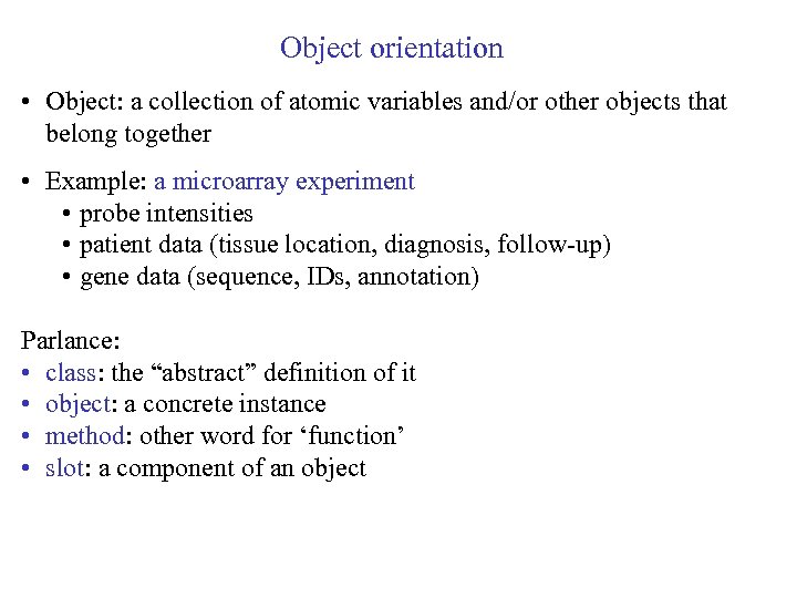Object orientation • Object: a collection of atomic variables and/or other objects that belong together • Example: a microarray experiment • probe intensities • patient data (tissue location, diagnosis, follow-up) • gene data (sequence, IDs, annotation) Parlance: • class: the “abstract” definition of it • object: a concrete instance • method: other word for ‘function’ • slot: a component of an object

Object orientation Advantages: Encapsulation (can use the objects and methods someone else has written without having to care about the internals) Generic functions (e. g. plot, print) Inheritance (hierarchical organization of complexity) Caveat: Overcomplicated, baroque program architecture…

variables > a = 49 > sqrt(a) [1] 7 > a = "The dog ate my homework" > sub("dog", "cat", a) [1] "The cat ate my homework“ > a = (1+1==3) >a [1] FALSE numeric character string logical

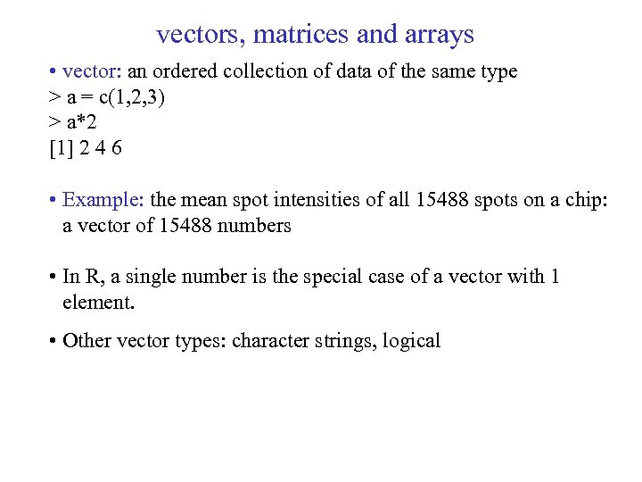vectors, matrices and arrays • vector: an ordered collection of data of the same type > a = c(1, 2, 3) > a*2 [1] 2 4 6 • Example: the mean spot intensities of all 15488 spots on a chip: a vector of 15488 numbers • In R, a single number is the special case of a vector with 1 element. • Other vector types: character strings, logical

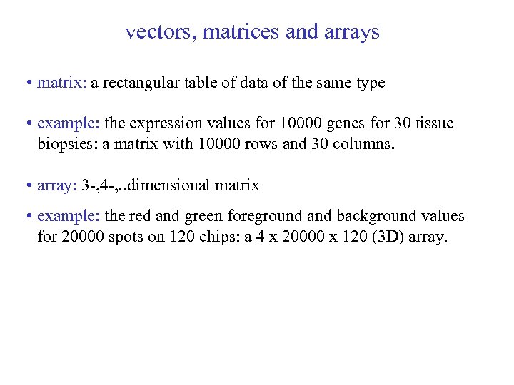vectors, matrices and arrays • matrix: a rectangular table of data of the same type • example: the expression values for 10000 genes for 30 tissue biopsies: a matrix with 10000 rows and 30 columns. • array: 3 -, 4 -, . . dimensional matrix • example: the red and green foreground and background values for 20000 spots on 120 chips: a 4 x 20000 x 120 (3 D) array.

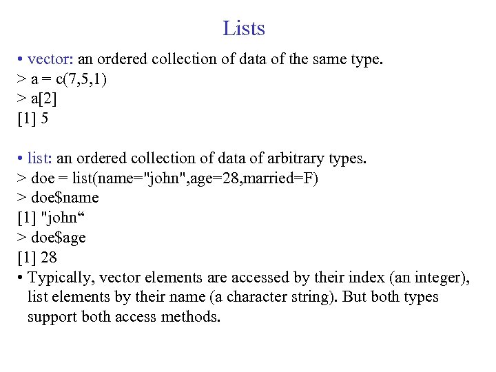Lists • vector: an ordered collection of data of the same type. > a = c(7, 5, 1) > a[2] [1] 5 • list: an ordered collection of data of arbitrary types. > doe = list(name="john", age=28, married=F) > doe$name [1] "john“ > doe$age [1] 28 • Typically, vector elements are accessed by their index (an integer), list elements by their name (a character string). But both types support both access methods.

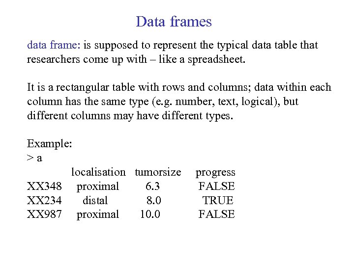Data frames data frame: is supposed to represent the typical data table that researchers come up with – like a spreadsheet. It is a rectangular table with rows and columns; data within each column has the same type (e. g. number, text, logical), but different columns may have different types. Example: >a localisation tumorsize XX 348 proximal 6. 3 XX 234 distal 8. 0 XX 987 proximal 10. 0 progress FALSE TRUE FALSE

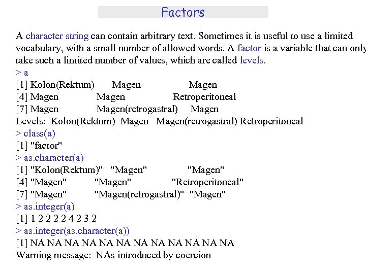Factors A character string can contain arbitrary text. Sometimes it is useful to use a limited vocabulary, with a small number of allowed words. A factor is a variable that can only take such a limited number of values, which are called levels. >a [1] Kolon(Rektum) Magen [4] Magen Retroperitoneal [7] Magen(retrogastral) Magen Levels: Kolon(Rektum) Magen(retrogastral) Retroperitoneal > class(a) [1] "factor" > as. character(a) [1] "Kolon(Rektum)" "Magen" [4] "Magen" "Retroperitoneal" [7] "Magen" "Magen(retrogastral)" "Magen" > as. integer(a) [1] 1 2 2 4 2 3 2 > as. integer(as. character(a)) [1] NA NA NA Warning message: NAs introduced by coercion

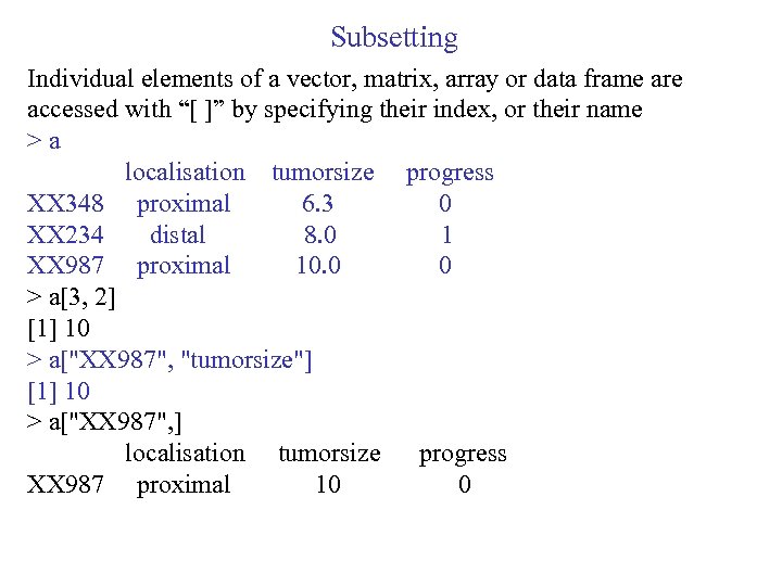Subsetting Individual elements of a vector, matrix, array or data frame are accessed with “[ ]” by specifying their index, or their name >a localisation tumorsize progress XX 348 proximal 6. 3 0 XX 234 distal 8. 0 1 XX 987 proximal 10. 0 0 > a[3, 2] [1] 10 > a["XX 987", "tumorsize"] [1] 10 > a["XX 987", ] localisation tumorsize progress XX 987 proximal 10 0

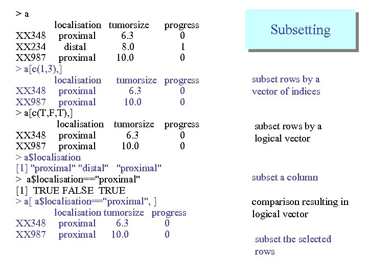>a localisation tumorsize progress XX 348 proximal 6. 3 0 XX 234 distal 8. 0 1 XX 987 proximal 10. 0 0 > a[c(1, 3), ] localisation tumorsize progress XX 348 proximal 6. 3 0 XX 987 proximal 10. 0 0 > a[c(T, F, T), ] localisation tumorsize progress XX 348 proximal 6. 3 0 XX 987 proximal 10. 0 0 > a$localisation [1] "proximal" "distal" "proximal" > a$localisation=="proximal" [1] TRUE FALSE TRUE > a[ a$localisation=="proximal", ] localisation tumorsize progress XX 348 proximal 6. 3 0 XX 987 proximal 10. 0 0 Subsetting subset rows by a vector of indices subset rows by a logical vector subset a column comparison resulting in logical vector subset the selected rows

Resources • A package specification allows the production of loadable modules for specific purposes, and several contributed packages are made available through the CRAN sites. • CRAN and R homepage: – http: //www. r-project. org/ It is R’s central homepage, giving information on the R project and everything related to it. – http: //cran. r-project. org/ It acts as the download area, carrying the software itself, extension packages, PDF manuals. • Getting help with functions and features – help(solve) – ? solve – For a feature specified by special characters, the argument must be enclosed in double or single quotes, making it a “character string”: help("[[")

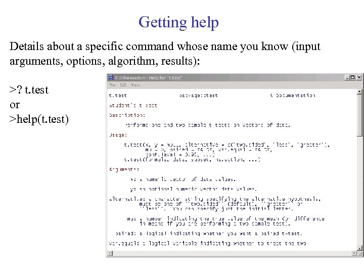Getting help Details about a specific command whose name you know (input arguments, options, algorithm, results): >? t. test or >help(t. test)

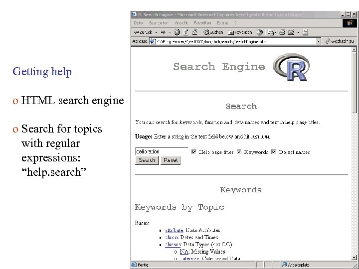Getting help o HTML search engine o Search for topics with regular expressions: “help. search”

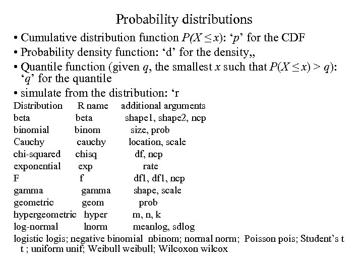Probability distributions • Cumulative distribution function P(X ≤ x): ‘p’ for the CDF • Probability density function: ‘d’ for the density, , • Quantile function (given q, the smallest x such that P(X ≤ x) > q): ‘q’ for the quantile • simulate from the distribution: ‘r Distribution R name additional arguments beta shape 1, shape 2, ncp binomial binom size, prob Cauchy cauchy location, scale chi-squared chisq df, ncp exponential exp rate F f df 1, ncp gamma shape, scale geometric geom prob hypergeometric hyper m, n, k log-normal lnorm meanlog, sdlog logistic logis; negative binomial nbinom; normal norm; Poisson pois; Student’s t t ; uniform unif; Weibull weibull; Wilcoxon wilcox

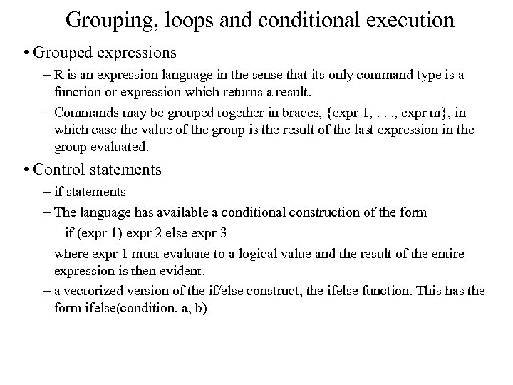Grouping, loops and conditional execution • Grouped expressions – R is an expression language in the sense that its only command type is a function or expression which returns a result. – Commands may be grouped together in braces, {expr 1, . . . , expr m}, in which case the value of the group is the result of the last expression in the group evaluated. • Control statements – if statements – The language has available a conditional construction of the form if (expr 1) expr 2 else expr 3 where expr 1 must evaluate to a logical value and the result of the entire expression is then evident. – a vectorized version of the if/else construct, the ifelse function. This has the form ifelse(condition, a, b)

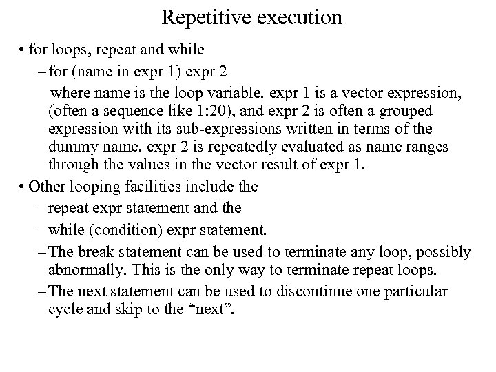Repetitive execution • for loops, repeat and while – for (name in expr 1) expr 2 where name is the loop variable. expr 1 is a vector expression, (often a sequence like 1: 20), and expr 2 is often a grouped expression with its sub-expressions written in terms of the dummy name. expr 2 is repeatedly evaluated as name ranges through the values in the vector result of expr 1. • Other looping facilities include the – repeat expr statement and the – while (condition) expr statement. – The break statement can be used to terminate any loop, possibly abnormally. This is the only way to terminate repeat loops. – The next statement can be used to discontinue one particular cycle and skip to the “next”.

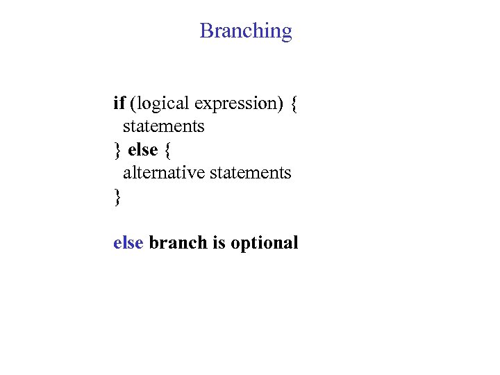Branching if (logical expression) { statements } else { alternative statements } else branch is optional

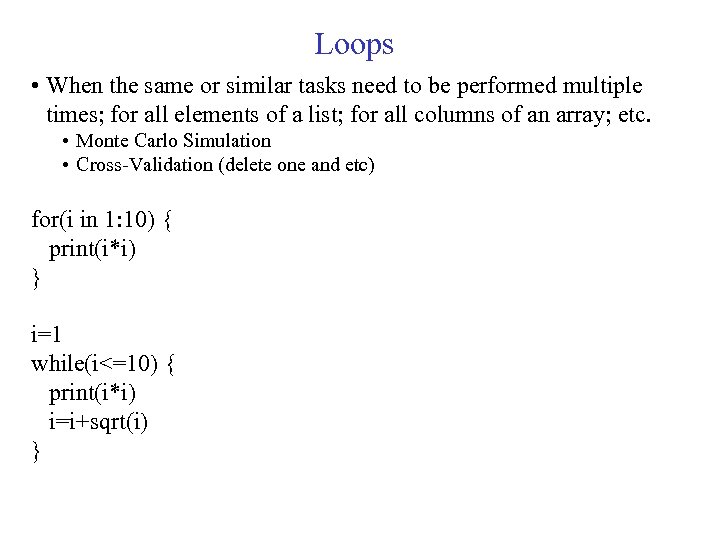Loops • When the same or similar tasks need to be performed multiple times; for all elements of a list; for all columns of an array; etc. • Monte Carlo Simulation • Cross-Validation (delete one and etc) for(i in 1: 10) { print(i*i) } i=1 while(i<=10) { print(i*i) i=i+sqrt(i) }

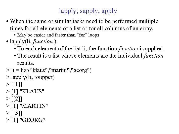lapply, sapply, apply • When the same or similar tasks need to be performed multiple times for all elements of a list or for all columns of an array. • May be easier and faster than “for” loops • lapply(li, function ) • To each element of the list li, the function is applied. • The result is a list whose elements are the individual function results. > li = list("klaus", "martin", "georg") > lapply(li, toupper) > [[1]] > [1] "KLAUS" > [[2]] > [1] "MARTIN" > [[3]] > [1] "GEORG"

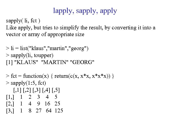lapply, sapply, apply sapply( li, fct ) Like apply, but tries to simplify the result, by converting it into a vector or array of appropriate size > li = list("klaus", "martin", "georg") > sapply(li, toupper) [1] "KLAUS" "MARTIN" "GEORG" > fct = function(x) { return(c(x, x*x*x)) } > sapply(1: 5, fct) [, 1] [, 2] [, 3] [, 4] [, 5] [1, ] 1 2 3 4 5 [2, ] 1 4 9 16 25 [3, ] 1 8 27 64 125

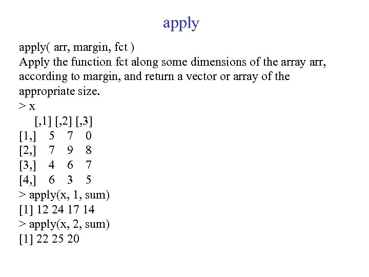apply( arr, margin, fct ) Apply the function fct along some dimensions of the array arr, according to margin, and return a vector or array of the appropriate size. >x [, 1] [, 2] [, 3] [1, ] 5 7 0 [2, ] 7 9 8 [3, ] 4 6 7 [4, ] 6 3 5 > apply(x, 1, sum) [1] 12 24 17 14 > apply(x, 2, sum) [1] 22 25 20

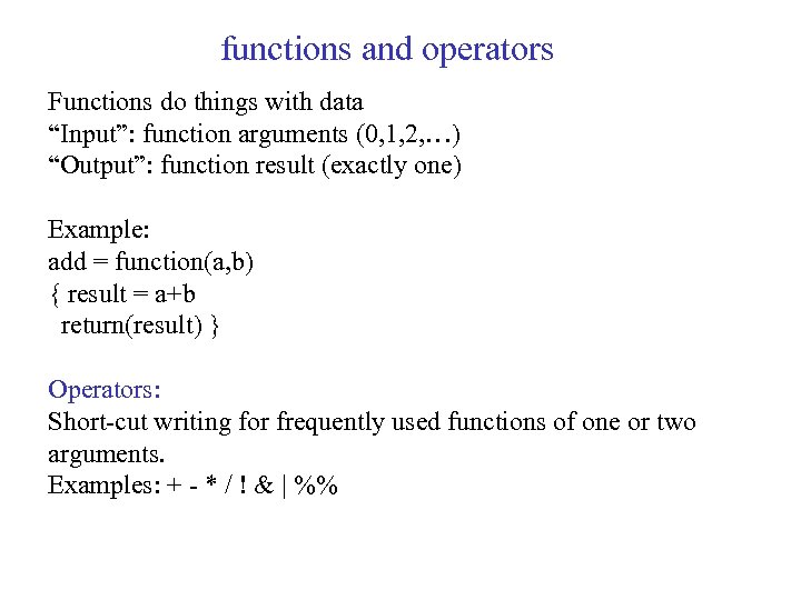functions and operators Functions do things with data “Input”: function arguments (0, 1, 2, …) “Output”: function result (exactly one) Example: add = function(a, b) { result = a+b return(result) } Operators: Short-cut writing for frequently used functions of one or two arguments. Examples: + - * / ! & | %%

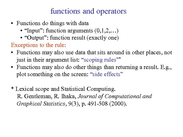functions and operators • Functions do things with data • “Input”: function arguments (0, 1, 2, …) • “Output”: function result (exactly one) Exceptions to the rule: • Functions may also use data that sits around in other places, not just in their argument list: “scoping rules”* • Functions may also do other things than returning a result. E. g. , plot something on the screen: “side effects” * Lexical scope and Statistical Computing. R. Gentleman, R. Ihaka, Journal of Computational and Graphical Statistics, 9(3), p. 491 -508 (2000).

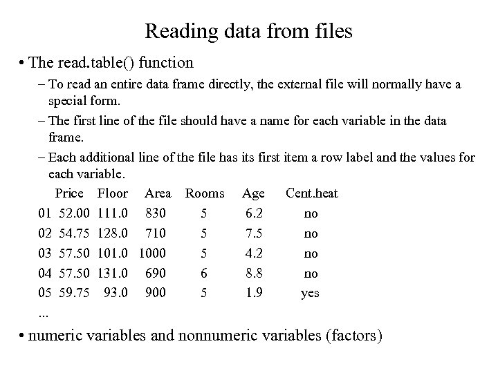Reading data from files • The read. table() function – To read an entire data frame directly, the external file will normally have a special form. – The first line of the file should have a name for each variable in the data frame. – Each additional line of the file has its first item a row label and the values for each variable. Price Floor Area Rooms Age Cent. heat 01 52. 00 111. 0 830 5 6. 2 no 02 54. 75 128. 0 710 5 7. 5 no 03 57. 50 101. 0 1000 5 4. 2 no 04 57. 50 131. 0 690 6 8. 8 no 05 59. 75 93. 0 900 5 1. 9 yes. . . • numeric variables and nonnumeric variables (factors)

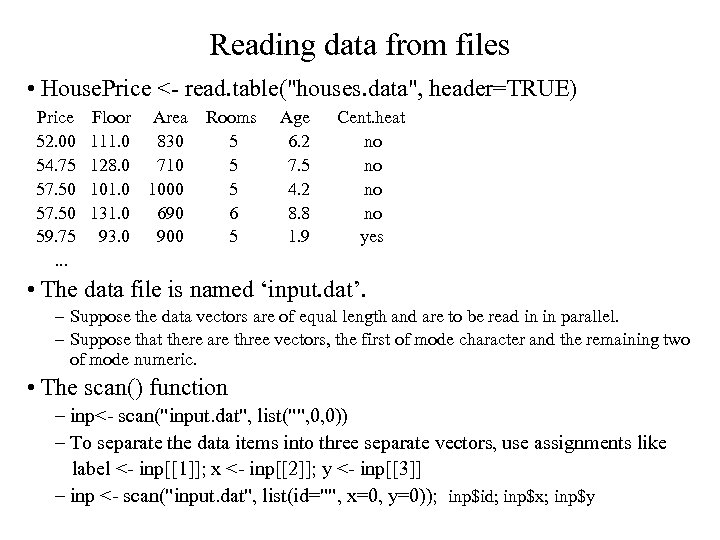Reading data from files • House. Price <- read. table("houses. data", header=TRUE) Price 52. 00 54. 75 57. 50 59. 75. . . Floor Area 111. 0 830 128. 0 710 101. 0 1000 131. 0 690 93. 0 900 Rooms 5 5 5 6 5 Age 6. 2 7. 5 4. 2 8. 8 1. 9 Cent. heat no no yes • The data file is named ‘input. dat’. – Suppose the data vectors are of equal length and are to be read in in parallel. – Suppose that there are three vectors, the first of mode character and the remaining two of mode numeric. • The scan() function – inp<- scan("input. dat", list("", 0, 0)) – To separate the data items into three separate vectors, use assignments like label <- inp[[1]]; x <- inp[[2]]; y <- inp[[3]] – inp <- scan("input. dat", list(id="", x=0, y=0)); inp$id; inp$x; inp$y

Storing data • Every R object can be stored into and restored from a file with the commands “save” and “load”. • This uses the XDR (external data representation) standard of Sun Microsystems and others, and is portable between MSWindows, Unix, Mac. > save(x, file=“x. Rdata”) > load(“x. Rdata”)

Importing and exporting data There are many ways to get data into R and out of R. Most programs (e. g. Excel), as well as humans, know how to deal with rectangular tables in the form of tab-delimited text files. > x = read. delim(“filename. txt”) also: read. table, read. csv > write. table(x, file=“x. txt”, sep=“t”)

Importing data: caveats Ø Type conversions: by default, the read functions try to guess and autoconvert the data types of the different columns (e. g. number, factor, character). Ø There are options as. is and col. Classes to control this – read the online help Ø Special characters: the delimiter character (space, comma, tabulator) and the end-of-line character cannot be part of a data field. Ø To circumvent this, text may be “quoted”. Ø However, if this option is used (the default), then the quote characters themselves cannot be part of a data field. Except if they themselves are within quotes… Ø Understand the conventions your input files use and set the quote options accordingly.

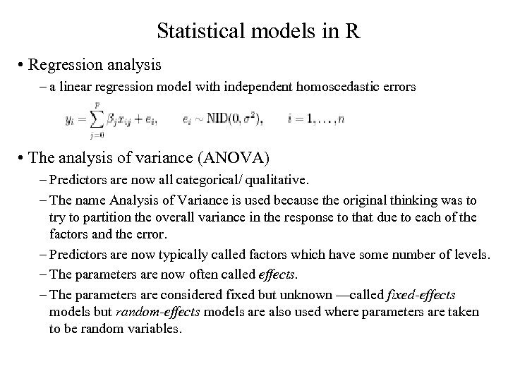Statistical models in R • Regression analysis – a linear regression model with independent homoscedastic errors • The analysis of variance (ANOVA) – Predictors are now all categorical/ qualitative. – The name Analysis of Variance is used because the original thinking was to try to partition the overall variance in the response to that due to each of the factors and the error. – Predictors are now typically called factors which have some number of levels. – The parameters are now often called effects. – The parameters are considered fixed but unknown —called fixed-effects models but random-effects models are also used where parameters are taken to be random variables.

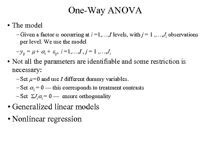One-Way ANOVA • The model – Given a factor a occurring at i =1, …, I levels, with j = 1 , …, Ji observations per level. We use the model – yij = µ+ ai + eij, i =1, …, I , j = 1 , …, Ji • Not all the parameters are identifiable and some restriction is necessary: – Set µ=0 and use I different dummy variables. – Set a 1 = 0 — this corresponds to treatment contrasts – Set SJiai = 0 — ensure orthogonality • Generalized linear models • Nonlinear regression

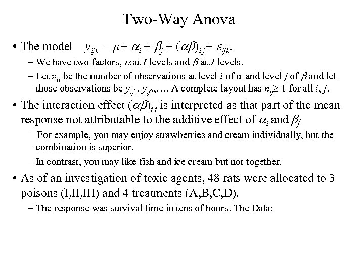Two-Way Anova • The model yijk = µ+ ai + bj + (ab)i j+ eijk. – We have two factors, a at I levels and b at J levels. – Let nij be the number of observations at level i of a and level j of b and let those observations be yij 1, yij 2, …. A complete layout has nij 1 for all i, j. • The interaction effect (ab)i j is interpreted as that part of the mean response not attributable to the additive effect of ai and bj. – For example, you may enjoy strawberries and cream individually, but the combination is superior. – In contrast, you may like fish and ice cream but not together. • As of an investigation of toxic agents, 48 rats were allocated to 3 poisons (I, III) and 4 treatments (A, B, C, D). – The response was survival time in tens of hours. The Data:

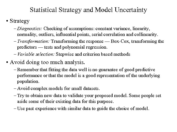Statistical Strategy and Model Uncertainty • Strategy – Diagnostics: Checking of assumptions: constant variance, linearity, normality, outliers, influential points, serial correlation and collinearity. – Transformation: Transforming the response — Box-Cox, transforming the predictors — tests and polynomial regression. – Variable selection: Stepwise and criterion based methods • Avoid doing too much analysis. – Remember that fitting the data well is no guarantee of good predictive performance or that the model is a good representation of the underlying population. – Avoid complex models for small datasets. – Try to obtain new data to validate your proposed model. Some people set aside some of their existing data for this purpose. – Use past experience with similar data to guide the choice of model.

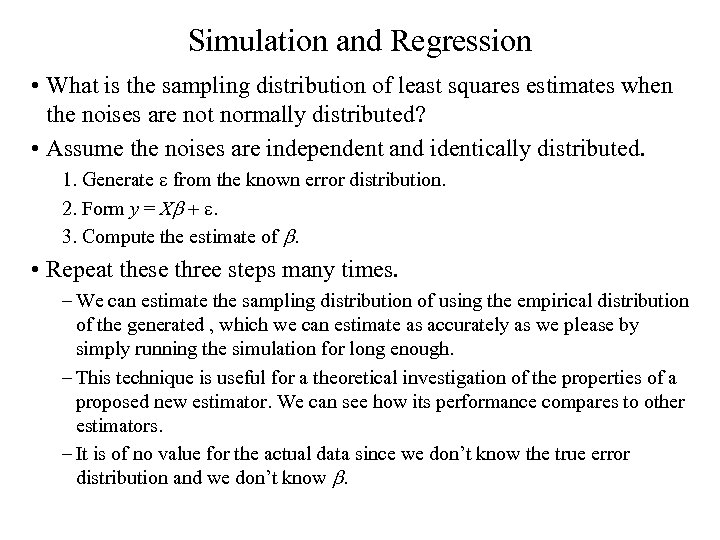Simulation and Regression • What is the sampling distribution of least squares estimates when the noises are not normally distributed? • Assume the noises are independent and identically distributed. 1. Generate e from the known error distribution. 2. Form y = Xb + e. 3. Compute the estimate of b. • Repeat these three steps many times. – We can estimate the sampling distribution of using the empirical distribution of the generated , which we can estimate as accurately as we please by simply running the simulation for long enough. – This technique is useful for a theoretical investigation of the properties of a proposed new estimator. We can see how its performance compares to other estimators. – It is of no value for the actual data since we don’t know the true error distribution and we don’t know b.

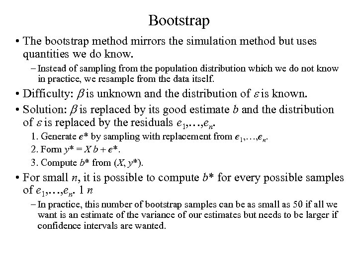Bootstrap • The bootstrap method mirrors the simulation method but uses quantities we do know. – Instead of sampling from the population distribution which we do not know in practice, we resample from the data itself. • Difficulty: b is unknown and the distribution of e is known. • Solution: b is replaced by its good estimate b and the distribution of e is replaced by the residuals e 1, …, en. 1. Generate e* by sampling with replacement from e 1, …, en. 2. Form y* = X b + e*. 3. Compute b* from (X, y*). • For small n, it is possible to compute b* for every possible samples of e 1, …, en. 1 n – In practice, this number of bootstrap samples can be as small as 50 if all we want is an estimate of the variance of our estimates but needs to be larger if confidence intervals are wanted.

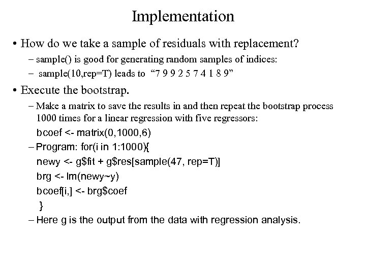Implementation • How do we take a sample of residuals with replacement? – sample() is good for generating random samples of indices: – sample(10, rep=T) leads to “ 7 9 9 2 5 7 4 1 8 9” • Execute the bootstrap. – Make a matrix to save the results in and then repeat the bootstrap process 1000 times for a linear regression with five regressors: bcoef <- matrix(0, 1000, 6) – Program: for(i in 1: 1000){ newy <- g$fit + g$res[sample(47, rep=T)] brg <- lm(newy~y) bcoef[i, ] <- brg$coef } – Here g is the output from the data with regression analysis.

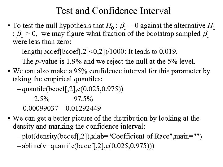Test and Confidence Interval • To test the null hypothesis that H 0 : b 1 = 0 against the alternative H 1 : b 1 > 0, we may figure what fraction of the bootstrap sampled b 1 were less than zero: – length(bcoef[, 2]<0, 2])/1000: It leads to 0. 019. – The p-value is 1. 9% and we reject the null at the 5% level. • We can also make a 95% confidence interval for this parameter by taking the empirical quantiles: – quantile(bcoef[, 2], c(0. 025, 0. 975)) 2. 5% 97. 5% 0. 00099037 0. 01292449 • We can get a better picture of the distribution by looking at the density and marking the confidence interval: – plot(density(bcoef[, 2]), xlab="Coefficient of Race", main="") – abline(v=quantile(bcoef[, 2], c(0. 025, 0. 975)))

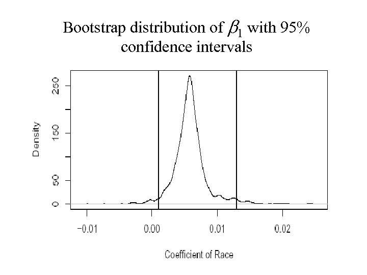Bootstrap distribution of b 1 with 95% confidence intervals

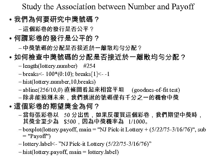Study the Association between Number and Payoff • 我們為何要研究中獎號碼？ – 這個彩卷的發行是否公平？ • 何謂彩卷的發行是公平的？ – 中獎號碼的分配是否接近於一離散均勻分配？ • 如何檢查中獎號碼的分配是否接近於一離散均勻分配？ – length(lottery. number) #254 – breaks<- 100*(0: 10); breaks[1]<- -1 – hist(lottery. number, 10, breaks) – abline(256/10, 0) 直條圖看起來相當平坦 (goodnes-of-fit test) – 除非能預測未來，我們挑選的號碼僅有千分之一的機會中獎 • 這個彩卷的期望獎金為何？ – 當每張彩卷以 50 分出售，如果反覆買這個彩卷，我們期望中獎時， 其獎金至少為 $500，因為中獎機率為 1/1000。 – boxplot(lottery. payoff, main = "NJ Pick-it Lottery + (5/22/75 -3/16/76)", sub = "Payoff") – lottery. label<- ”NJ Pick-it Lottery (5/22/75 -3/16/76)” – hist(lottery. payoff, main = lottery. label)

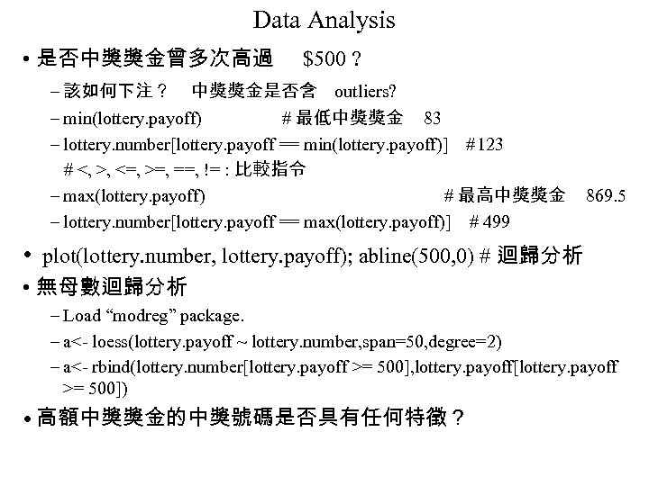Data Analysis • 是否中獎獎金曾多次高過 $500 ? – 該如何下注？ 中獎獎金是否含 outliers? – min(lottery. payoff) # 最低中獎獎金 83 – lottery. number[lottery. payoff == min(lottery. payoff)] #123 # <, >, <=, >=, ==, != : 比較指令 – max(lottery. payoff) # 最高中獎獎金 – lottery. number[lottery. payoff == max(lottery. payoff)] # 499 869. 5 • plot(lottery. number, lottery. payoff); abline(500, 0) # 迴歸分析 • 無母數迴歸分析 – Load “modreg” package. – a<- loess(lottery. payoff ~ lottery. number, span=50, degree=2) – a<- rbind(lottery. number[lottery. payoff >= 500], lottery. payoff[lottery. payoff >= 500]) • 高額中獎獎金的中獎號碼是否具有任何特徵？

高額中獎獎金的中獎號碼特徵 • 特徵：大部份高額獎金中獎號碼，都有重複的數字。 – 此彩卷有一特別下注的方式稱作「 combination bets」， 下注號碼必須 是三個不同的數字，只要下注號碼與中獎號碼中所含的數字相同 就算中獎。 – plot(a[1, ], a[2, ], xlab="lottery. number", ylab="lottery. payoff", main= "Payoff >=500") – boxplot(split(lottery. payoff, lottery. number%/%100), sub= "Leading Digit of Winning Numbers", ylab= "Payoff") 依據中獎號碼的首位數字製作盒狀圖。 當中獎號碼的首位數字為零時，其獎金都較高。一個解釋是較少 人會下注這樣的號碼。 • 在不同時間下，中獎獎金金額的比較。 – qqplot(lottery. payoff, lottery 3. payoff); abline(0, 1) – 使用盒狀圖來比較不同時間下，中獎獎金金額的分配。 – boxplot(lottery. payoff, lottery 2. payoff, lottery 3. payoff) – 依時間先後來看，中獎獎金金額漸漸穩定下來，很少能超過 $500。 – rbind(lottery 2. number[lottery 2. payoff >= 500], lottery 2. payoff[lottery 2. payoff >= 500]) – rbind(lottery 3. number[lottery 3. payoff >= 500], lottery 3. payoff[lottery 3. payoff >= 500])

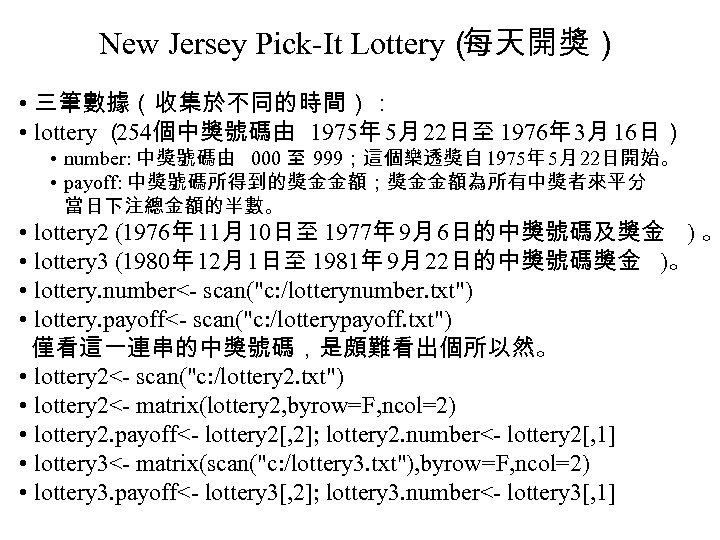New Jersey Pick-It Lottery（ 每天開獎） • 三筆數據（收集於不同的時間）： • lottery （ 254個中獎號碼由 1975年 5月 22日至 1976年 3月 16日） • number: 中獎號碼由 000 至 999；這個樂透獎自 1975年 5月 22日開始。 • payoff: 中獎號碼所得到的獎金金額；獎金金額為所有中獎者來平分 當日下注總金額的半數。 • lottery 2 (1976年 11月 10日至 1977年 9月 6日的中獎號碼及獎金 ) 。 • lottery 3 (1980年 12月 1日至 1981年 9月 22日的中獎號碼獎金 )。 • lottery. number<- scan("c: /lotterynumber. txt") • lottery. payoff<- scan("c: /lotterypayoff. txt") 僅看這一連串的中獎號碼，是頗難看出個所以然。 • lottery 2<- scan("c: /lottery 2. txt") • lottery 2<- matrix(lottery 2, byrow=F, ncol=2) • lottery 2. payoff<- lottery 2[, 2]; lottery 2. number<- lottery 2[, 1] • lottery 3<- matrix(scan("c: /lottery 3. txt"), byrow=F, ncol=2) • lottery 3. payoff<- lottery 3[, 2]; lottery 3. number<- lottery 3[, 1]

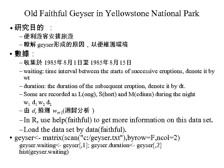Old Faithful Geyser in Yellowstone National Park • 研究目的 ： – 便利遊客安排旅遊 – 瞭解 geyser形成的原因，以便維護環境 • 數據： – 收集於 1985年 8月 1日至 1985年 8月 15日 – waiting: time interval between the starts of successive eruptions, denote it by wt – duration: the duration of the subsequent eruption, denote it by dt. – Some are recorded as L(ong), S(hort) and M(edium) during the night w 1 d 1 w 2 d 2 – 由 dt 預測 wt+1(迴歸分析 ) – In R, use help(faithful) to get more information on this data set. – Load the data set by data(faithful). • geyser<- matrix(scan("c: /geyser. txt"), byrow=F, ncol=2) geyser. waiting<- geyser[, 1]; geyser. duration<- geyser[, 2] hist(geyser. waiting)

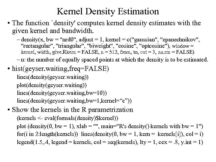Kernel Density Estimation • The function `density' computes kernel density estimates with the given kernel and bandwidth. – density(x, bw = "nrd 0", adjust = 1, kernel = c("gaussian", "epanechnikov", "rectangular", "triangular", "biweight", "cosine", "optcosine"), window = kernel, width, give. Rkern = FALSE, n = 512, from, to, cut = 3, na. rm = FALSE) – n: the number of equally spaced points at which the density is to be estimated. • hist(geyser. waiting, freq=FALSE) lines(density(geyser. waiting)) plot(density(geyser. waiting)) lines(density(geyser. waiting, bw=10)) lines(density(geyser. waiting, bw=1, kernel=“e”)) • Show the kernels in the R parametrization (kernels <- eval(formals(density)$kernel)) plot (density(0, bw = 1), xlab = "", main="R's density() kernels with bw = 1") for(i in 2: length(kernels)) lines(density(0, bw = 1, kern = kernels[i]), col = i) legend(1. 5, . 4, legend = kernels, col = seq(kernels), lty = 1, cex =. 8, y. int = 1)

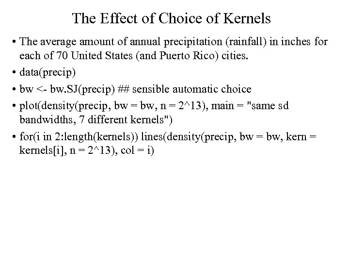The Effect of Choice of Kernels • The average amount of annual precipitation (rainfall) in inches for each of 70 United States (and Puerto Rico) cities. • data(precip) • bw <- bw. SJ(precip) ## sensible automatic choice • plot(density(precip, bw = bw, n = 2^13), main = "same sd bandwidths, 7 different kernels") • for(i in 2: length(kernels)) lines(density(precip, bw = bw, kern = kernels[i], n = 2^13), col = i)

迴歸分析 • duration<- geyser. duration[1: 298] • waiting<- geyser. waiting[2: 299] • plot(duration, waiting, xlab="噴泉持續時間 ", ylab="waiting") • plot(density(duration), xlab="噴泉持續時間 ", ylab="density") plot(density(geyser. waiting), xlab="waiting", ylab="density") • # 由 wt 預測 dt • plot(geyser. waiting, geyser. duration, xlab="waiting", ylab="duration") • 可能之物理模型 • 噴泉口之下方有一細長 tube， 內充滿了水而受環繞岩石加熱。 由於 tube內滿了大量的水，故 tube下方的水因壓力的緣故，其沸點較高， 且愈深處沸點愈高。 • 當 tube上方的水，因環繞岩石加熱達到沸點變為蒸氣；而較下方的水因 壓力降低，故其沸點隨之降低，而加速將下方的水變為蒸氣，故開始噴 泉。 • 有關此物理模型之進一步討論，參看 Rinehart (1969; J. Geophy. Res. , 566573)

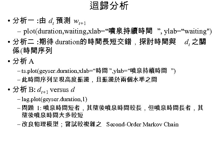迴歸分析 • 分析一 : 由 dt 預測 wt+1 – plot(duration, waiting, xlab=“噴泉持續時間 ”, ylab=“waiting") • 分析二 : 期待 duration的時間長短交錯，探討時間與 dt 之關 係 (時間序列 • 分析 A – ts. plot(geyser. duration, xlab=“時間 ”, ylab=“噴泉持續時間 ”) – 此時間序列呈現高度振盪，且振盪於兩個水準之間 • 分析 B: dt+1 versus d – lag. plot(geyser. duration, 1) – 問題 1: 噴泉時間短者，其隨後噴泉時間較長，但噴泉時間長者，其 隨後噴泉時間大多較短 – 改良物理模型；嘗試較複雜之 Second-Order Markov Chain

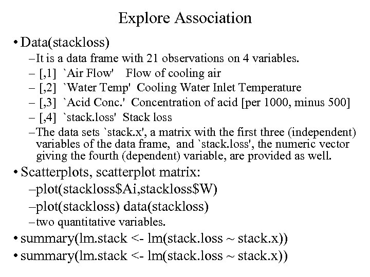Explore Association • Data(stackloss) – It is a data frame with 21 observations on 4 variables. – [, 1] `Air Flow' Flow of cooling air – [, 2] `Water Temp' Cooling Water Inlet Temperature – [, 3] `Acid Conc. ' Concentration of acid [per 1000, minus 500] – [, 4] `stack. loss' Stack loss – The data sets `stack. x', a matrix with the first three (independent) variables of the data frame, and `stack. loss', the numeric vector giving the fourth (dependent) variable, are provided as well. • Scatterplots, scatterplot matrix: –plot(stackloss$Ai, stackloss$W) –plot(stackloss) data(stackloss) – two quantitative variables. • summary(lm. stack <- lm(stack. loss ~ stack. x))

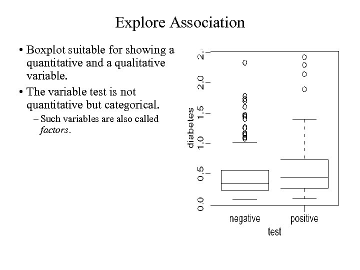Explore Association • Boxplot suitable for showing a quantitative and a qualitative variable. • The variable test is not quantitative but categorical. – Such variables are also called factors.

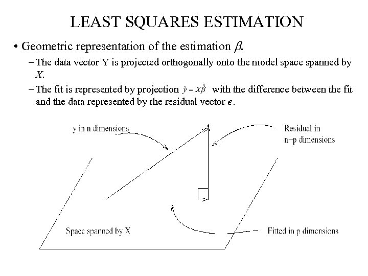LEAST SQUARES ESTIMATION • Geometric representation of the estimation b. – The data vector Y is projected orthogonally onto the model space spanned by X. – The fit is represented by projection with the difference between the fit and the data represented by the residual vector e.

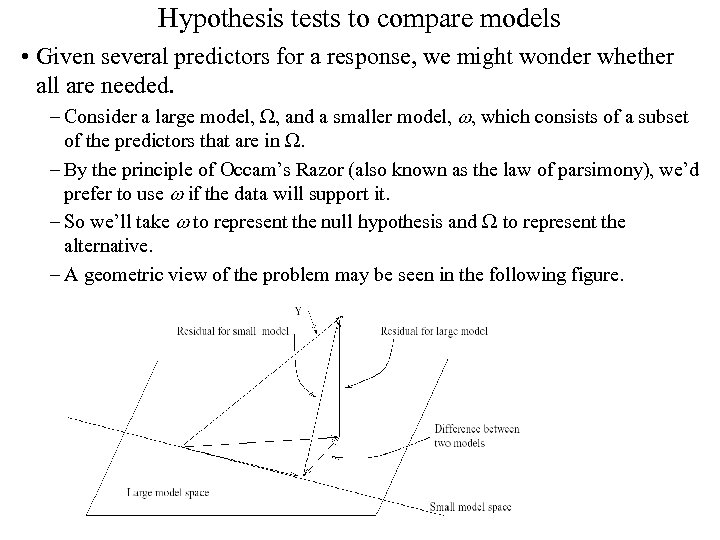Hypothesis tests to compare models • Given several predictors for a response, we might wonder whether all are needed. – Consider a large model, W, and a smaller model, w, which consists of a subset of the predictors that are in W. – By the principle of Occam’s Razor (also known as the law of parsimony), we’d prefer to use w if the data will support it. – So we’ll take w to represent the null hypothesis and W to represent the alternative. – A geometric view of the problem may be seen in the following figure.