b612ee9767285f6e07b4797e116e6156.ppt
- Количество слайдов: 156


QUEUING THEORY q Body of knowledge about waiting lines q Helps managers to better understand systems in manufacturing, service, and maintenance q Provides competitive advantage and cost saving A QUEUE REPRESENTS ITEMS OR PEOPLE AWAITING SERVICE Applied Management Science for Decision Making, 1 e © 2012 Pearson Prentice-Hall, Inc. Philip A. Vaccaro , Ph. D

Queue Characteristics Ø Average number of customers in a line Ø Average number of customers in a service facility Ø Probability a customer must wait Ø Average time a customer spends in a waiting line. Ø Average time a customer spends in a service facility Ø Percentage of time a service facility is busy

Queuing System Examples System Customers Servers Grocery Store Shoppers Checkout Clerks Phone System Phone Calls Switching Equipment Toll Highway Vehicles Tollgate Restaurant Parties of Diners Tables & Waitstaff Factory Products Workers

The Father of Queuing Theory Danish engineer, who, in 1909 experimented with fluctuating demand in telephone traffic in Copenhagen. In 1917, he published a report addressing the delays in automatic telephone dialing equipment. At the end of World War II, his work was extended to more general problems, including waiting lines in business. AGNER K. ERLANG

Lack of Managerial Intuition Surrounding Waiting Lines Queuing theory is not a matter of common sense. It is one of those applications where diligent, intelligent managers will arrive at drastically wrong solutions if they fail to thoroughly appreciate and understand the mathematics involved.

THE QUEUING COST TRADE-OFF Cost Total Cost of Providing Service Minimum Total Cost ( salaries + benefits ) Cost of Waiting Time ( time x value of time ) Low Level Of Service Optimal Service Level High Level Of Service

Aspects of a Queuing Process n SYSTEM ARRIVALS n THE QUEUE ITSELF n THE SERVICE FACILITY

The Calling Population q The source of all system arrivals q It is usually of infinite size q Theoretically, any person or object can enter the service facility during operating hours
 . 25 Poisson Probability Distribution for λ=2")
Poisson Arrival Distribution P ( probability ) . 25 Poisson Probability Distribution for λ=2 (estimated mean arrival rate) . 20. 15. 10. 05. 00 0 1 2 3 4 5 6 7 8 9 10 X ( the number of arrivals )
 . 25 Poisson Probability Distribution for λ=4")
Poisson Arrival Distribution P ( probability ) . 25 Poisson Probability Distribution for λ=4 (estimated mean arrival rate) . 20. 15. 10. 05. 00 0 1 2 3 4 5 6 7 8 9 10 X ( the number of arrivals )
")
Establishing A Discrete Poisson Arrival Distribution Given any average arrival rate ( λ ) in seconds, minutes, hours, days: P(X) = -λ ε λ X! x ( FOR X = 0, 1, 2, 3, 4, 5, etc. ) Where : P ( X ) = X = λ = ε = probability of X arrivals number of arrivals per time unit the average arrival rate 2. 7183 ( base of the natural logarithm )

EXAMPLE If the average arrival rate per hour is two people ( λ = 2 ) , what is the probability of three ( 3 ) arrivals per hour?
 = ε λ X! Given λ = 2 : -2")
Solution X -λ P(X) = ε λ X! Given λ = 2 : -2 P ( 3 ) = 2. 7183 3! 3 2 = [ 1 / 7. 389 ] x 8 (3)(2)(1) =. 1353 x 8 =. 1804 ≈ 18% 6
 =")
The Remaining Probabilities GIVEN THAT λ = 2 P ( 0 arrivals ) = P ( 1 arrival ) = P ( 2 arrivals ) = P ( 3 arrivals ) = P ( 4 arrivals ) = P ( 5 arrivals ) = P ( 6 arrivals ) = P ( 7 arrivals ) = P ( 8 arrivals ) = P ( 9 arrivals ) = P ( => 10 “ ) = 14% 28% 18% 9% 4% 2% 1%. 8%. 6% 0%

Poisson Probability Table For a given value of λ , entry indicates the probability of obtaining a specified value of ‘X’ X λ = 1. 8 λ = 1. 9 λ = 2. 0 0 . 1653 . 1496 . 1353 1 . 2975 . 2842 . 2707 2 . 2678 . 2700 . 2707 3 . 1607 . 1710 . 1804 4 . 0723 . 0812 . 0902 5 . 0260 . 0309 . 0361 6 . 0078 . 0098 . 0120 7 . 0020 . 0027 . 0034 8 . 0005 . 0006 . 0009 9 . 0001 . 0002 EXAMPLE

Precise Terminology Theoretical Distribution Observed Distribution The discrete arrival probability distribution, based on the average arrival rate ( λ ) which was computed from the actual system observations The actual discrete arrival probability distribution that was constructed from the actual system observations THIS DISTRIBUTION MAY OR MAY NOT BE POISSON DISTRIBUTED.

The theoretical poisson arrival probability distribution must be statistically identical to the observed arrival probability distribution THIS CAN BE ESTABLISHED BY A GOODNESS – OF - FIT HYPOTHESIS TEST If the two probability distributions are not found to be statistically identical, we are forced to study and solve the problem via simulation modeling

Service Times P R O B A B I L I T Y . 25. 20. 15 THE PROBABILITY A CUSTOMER WILL REQUIRE THAT SERVICE TIME . 10. 05. 00 0 30 60 90 120 150 180 210 seconds Service times normally follow a negative exponential probability distribution

Queue Discipline q Balking, reneging, and jockeying are not permitted in the service system. q Jockeying is the switching from one waiting line to another. JOCKEYING CAN BE DISCOURAGED BY PLACING BARRICADES SUCH AS MAGAZINE RACKS AND IMPULSE ITEM DISPLAYS BETWEEN WAITING LINES
 is the average arrival rate of")
Queuing Theory Variables n Lambda ( λ ) is the average arrival rate of people or items into the service system. n It can be expressed in seconds, minutes, hours, or days. n From the Greek small letter “ L “.
 is the average service rate of")
Queuing Theory Variables n Mu ( μ ) is the average service rate of the service system. n It can be expressed as the number of people or items processed per second, minute, hour, or day. n From the Greek small letter “ M “.
 is the % of")
Queuing Theory Variables n n § Rho ( ρ ) is the % of time that the service facility is busy on the average. It is also known as the utilization rate. From the Greek small letter “ R “. “BUSY” IS DEFINED AS AT LEAST ONE PERSON OR ITEM IN THE SYSTEM
 is a channel or service point")
Queuing Theory Variables n Mu ( M ) is a channel or service point in the service system. n Examples are gasoline pumps, checkout counters, vending machines, bank teller windows. n From the Greek large letter “ M “.

Queuing Theory Variables n Phases are the number of service points that must be negotiated by a customer or item before leaving the service system. n They have no symbol. A CARWASH TAKES A VEHICLE THROUGH SEVERAL PHASES: PRE-WASH, WAX, AND DRY BEFORE IT IS ALLOWED TO LEAVE THE FACILITY.
 is the percentage")
Queuing Theory Variables • Po or ( 1 – ρ ) is the percentage of time that the service facility is idle. • L is the average number of people or items in the service system both waiting to be served and currently being served. • Lq is the average number of people or items in the waiting line ( queue ) only !

Queuing Theory Variables • W is the average time a customer or item spends in the service system, both waiting and receiving service. • Wq is the average time a customer or item spends in the waiting line ( queue ) only. • Pw is the probability that a customer or item must wait to be served.

Queuing Theory Variables “Mμ” is the effective service rate. * The average number of customers or items processed by the entire service system It can be expressed in seconds, minutes, hours, or days * [ NUMBER OF SERVERS ] x [ AVERAGE SERVICE RATE PER SERVER ]

IMPORTANT CONSIDERATION n The average service rate must always exceed the average arrival rate. n Otherwise, the queue will grow to infinity. THERE WOULD BE NO SOLUTION ! μ>λ

Single-Channel / Single-Phase System EXIT q ONE WAITING LINE or QUEUE q ONE SERVICE POINT or CHANNEL

Dual-Channel / Single-Phase System EXIT q ONE OR TWO WAITING LINES q TWO DUPLICATE SERVICE POINTS EXIT No Jockeying Permitted Between Lines

Dual-Channel / Triple-Phase System EXIT C C B B A A ENTER q TWO IDENTICAL SERVICE CHANNELS. q EACH CHANNEL HAS 3 DISTINCT SERVICE POINTS ( A-B-C ) EXIT Jockeying Is Permitted Between Lines !

The Service System COMPRISED OF TWO GROUPS Customers or items waiting to be served or processed SUPERMARKET SHOPPERS ARE NOT IN THE SERVICE SYSTEM UNTIL THEY MOVE TO THE CHECKOUT AREA RESTAURANT PATRONS ENTER THE SERVICE SYSTEM AS SOON AS THEY ARRIVE Customers or items currently being served or processed
 channels and / or")
Queuing Theory Limitations Formulae only accommodate eight ( 8 ) channels and / or eight ( 8 ) phases If service systems exceed the above, it may be possible to divide them into sub-systems for separate analyses. BJ’s WHOLESALE CLUB HAS FOURTEEN (14) CHECKOUTS. HOWEVER, THEY COULD BE DIVIDED INTO CONTRACTOR, EXPRESS, CASH-ONLY, AND CREDIT-CARD-ONLY SUBSYSTEMS.

Stealth Queuing Systems NORMAL CHARACTERISTICS MISSING VISITING NURSES, PLUMBERS, ELECTRICIANS Moving waiting lines may be replaced by sitting customers or stockpiled items. Fixed channels may be replaced by mobile servers who carry portable equipment and make housecalls. BROKEN MACHINES WAITING FOR A MECHANIC, OR SEATED PATIENTS IN A DENTIST’S OFFICE, OR WORK-IN-PROCESS INVENTORY WAITING FOR PROCESSING.

Behavioral Considerations QUEUING THEORY n Customer willingness to wait depends on what is perceived as reasonable. n Waiting lines that are always moving are perceived as less painful. n Customer willingness to wait is higher if they know that others are also waiting their turn. n Customers should be permitted to perform the services that they can easily provide for themselves.

Behavioral Considerations QUEUING THEORY n n Well projected waiting times allow customers to adjust their expectations and therefore their aggravation. If customers are kept busy, their waiting time may not be construed as wasted time. FILLING OUT SURVEYS AND FORMS, BEING ENTERTAINED n Customers should be rewarded with price discounts or gifts if they must wait beyond a certain period of time. IT SHOWS THAT THE FIRM VALUES THEIR TIME AND IS WILLING TO PAY THEM FOR IT IF THE WAIT IS TOO LONG

Single-Channel / Single-Phase Model The Average Number of Customers in the System λ L = μ - λ

Single-Channel / Single-Phase Model The Average Number Just Waiting in Line λ Lq = 2 μ(μ- λ)

Single-Channel / Single-Phase Model Average Customer Time Spent in the System 1 W = (μ- λ)

Single-Channel / Single-Phase Model Percentage of Time the System is Busy λ ρ = μ

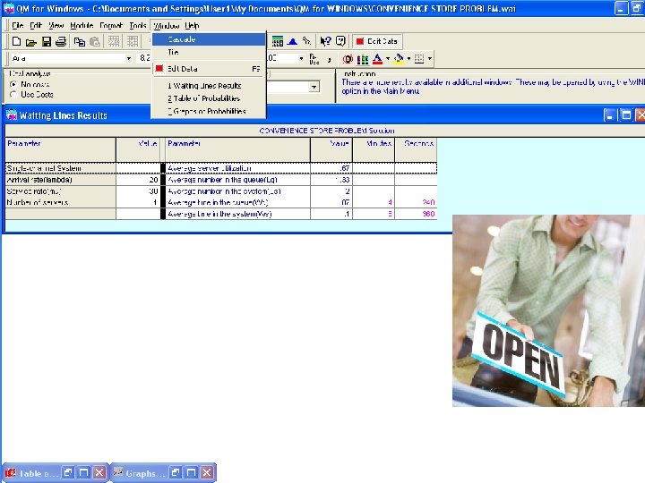
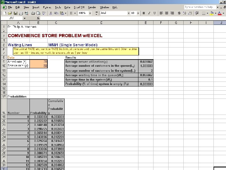
Single-Channel / Single-Phase Model APPLICATION n A clerk can serve thirty customers per hour on average. Therefore: μ = 30 λ = 20 n Twenty customers arrive each hour on average. M= 1

Single-Channel / Single-Phase Model APPLICATION The Average Number of Customers in the System 20 L = ( 30 - 20 ) = 2

Single-Channel / Single-Phase Model APPLICATION The Average Number Just Waiting in Line ( 20 ) Lq = 2 30 ( 30 - 20 ) = 1. 33

Single-Channel / Single-Phase Model APPLICATION The Average Customer Time Spent in the System W = 1 ( 30 - 20 ) =. 10 hrs ( 6 minutes )

Single-Channel / Single-Phase Model APPLICATION The Percentage of Time the System is Busy ρ = 20 30 = 67%

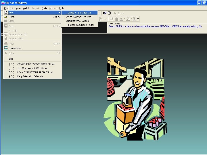
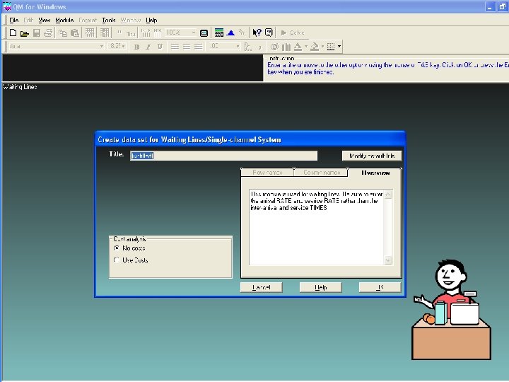
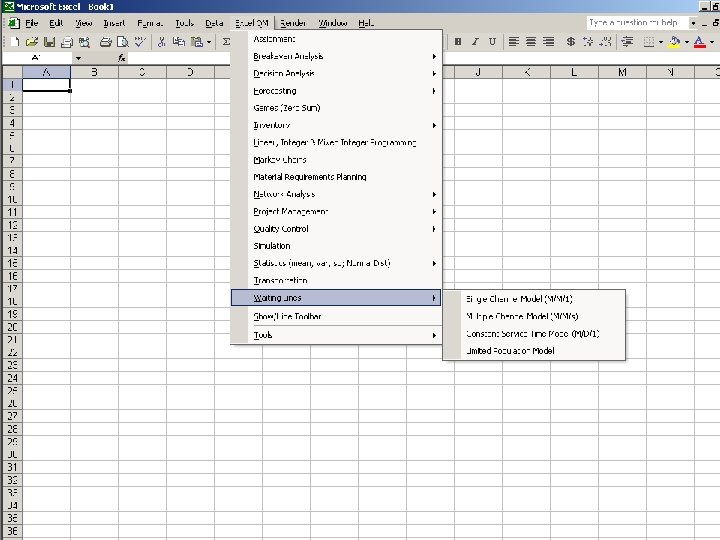
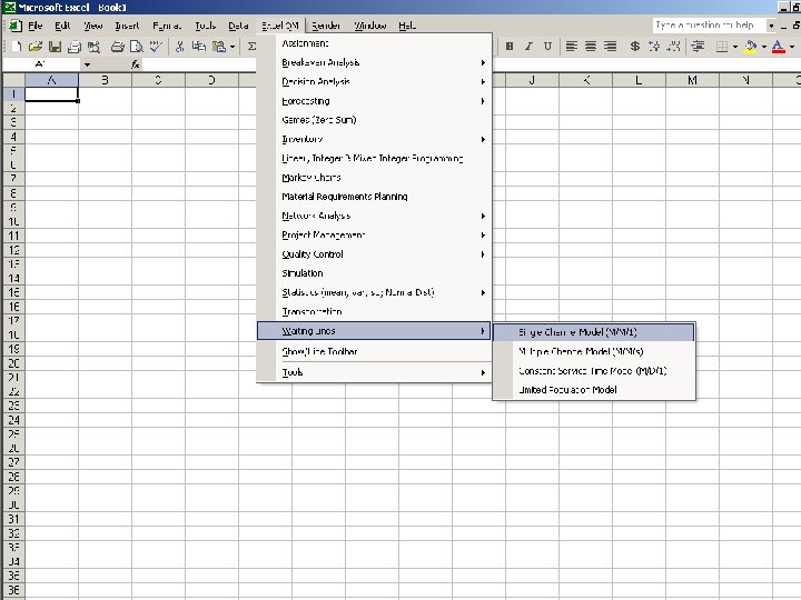
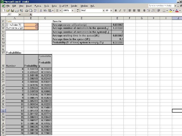
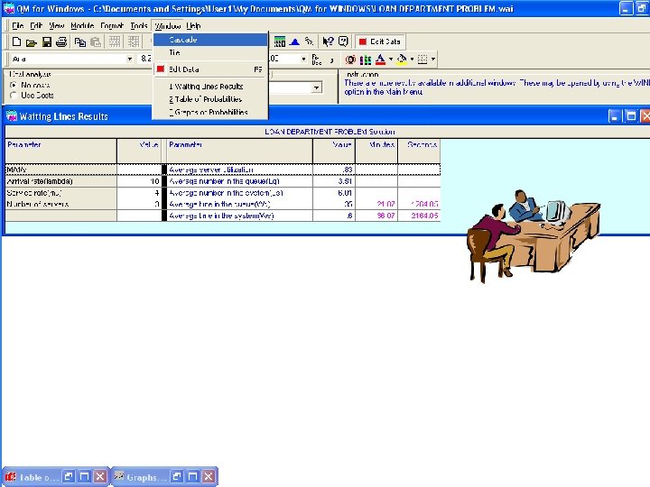
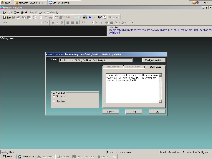
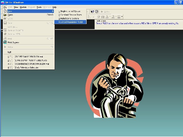
QM for Windows QUEUING APPLICATIONS Single-Channel Single-Phase Model

WE SCROLL TO “WAITING LINES”
 Clerk On-Duty Twenty ( 20 ) Arrivals per Hour Thirty")
One ( 1 ) Clerk On-Duty Twenty ( 20 ) Arrivals per Hour Thirty ( 30 ) Customers Can Be Served per Hour
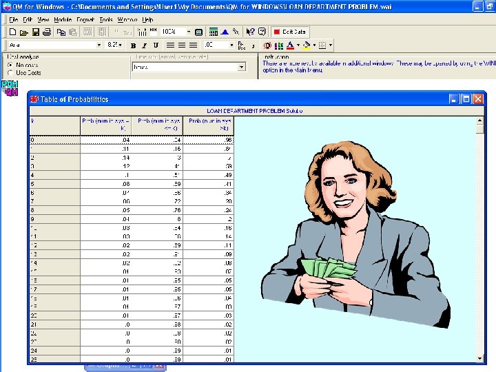
 persons in the system is 2% (=k) The")
The probability of exactly seven (7) persons in the system is 2% (=k) The probability of seven or fewer persons in the system is 96% ( <= k ) The probability of more than seven (7) persons in the system is 4% (>k)

Queuing Theory Modeling with Single-Channel Single-Phase Model
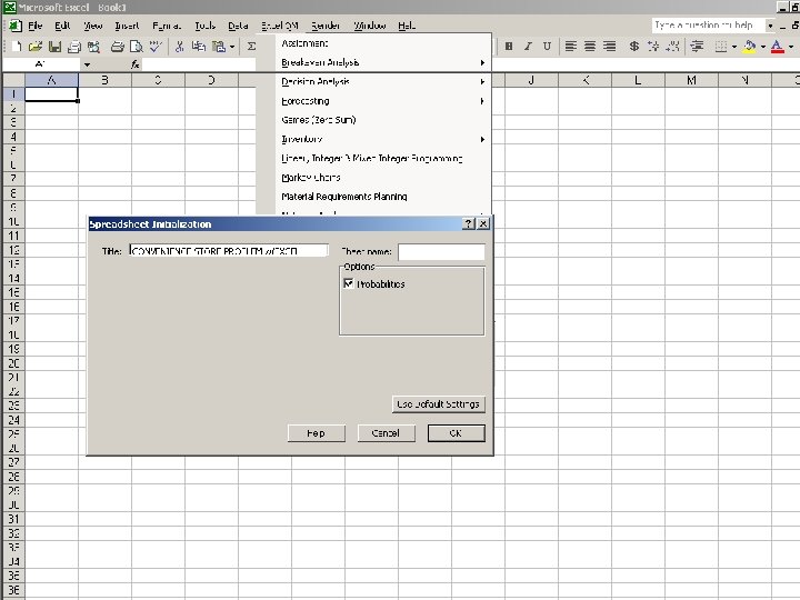

Template and Sample Data

Multi-Channel Single-Phase Systems This system is a single waiting line serviced by more than one server. It assumes: ü an infinite calling population ü a first-come, first-served queue discipline ü a poisson arrival rate ü negative exponential service times Additional Parameters M = number of servers or channels Mμ = mean effective service rate for the facility

Multi-Channel Single-Phase Systems The probability that the service facility is idle: 1 Po = n = M-1 n Σ 1/n! (λ / μ) n=0 + 1 M! M (λ / μ). Mμ Mμ-λ

Multi-Channel Single-Phase Systems The average number of customers in the system: λμ ( λ / μ ) L= M (M-1)! (Mμ-λ) 2 . Po + λ / μ

Multi-Channel Single-Phase Systems The average number of customers in the queue: Lq = L – ( λ / μ ) The average time a customer spends in the system: W=L/λ The average waiting time in the queue: Wq = W – ( 1 / μ ) or Lq / λ The probability that all the system’s servers are currently busy: M Pw = 1 M! λ μ . Mμ Mμ-λ . Po

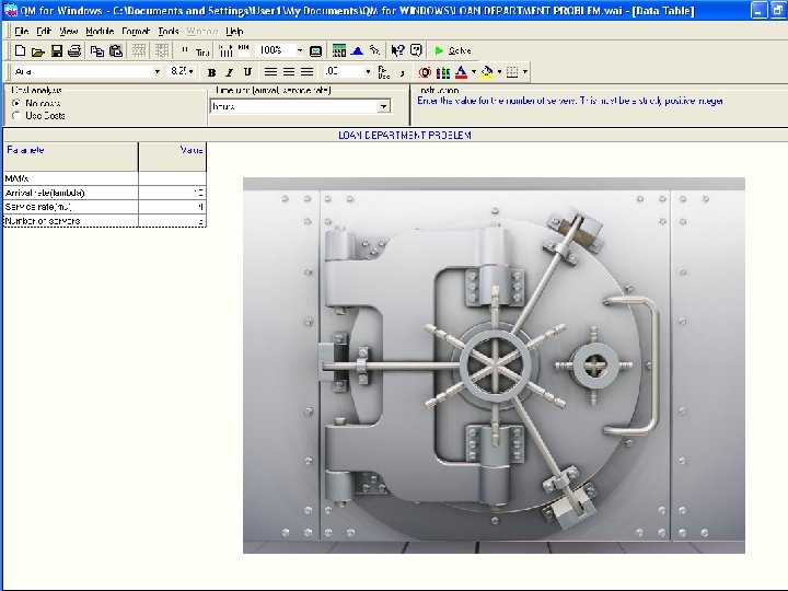
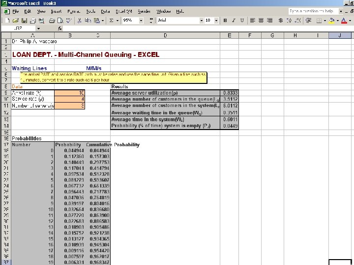
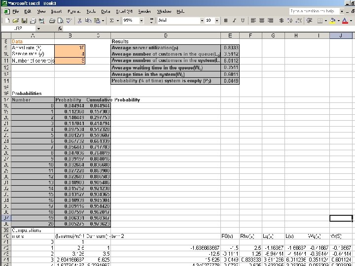
Multi-Channel Single-Phase Systems Application Example A bank has three loan officers on duty, each of whom can serve four customers per hour. Every hour, ten loan applicants arrive at the loan department and join a common queue. What are the system’s operating characteristics? 1 Po = 0 1 2 1 (10 / 4 ) + 1 ( 10 / 4 ) 0! 1! 2! =. 045 = 4. 5% 3 + 1. ( 10 / 4 ). 3! 3(4) - 10
( 4 )( 10 /")
Multi-Channel Single-Phase Systems Application Example Continued L= ( 10 )( 4 )( 10 / 4 ) 3 . (. 045 ) + [ 10 / 4 ] = 2 ( 3 – 1 ) ! [ 3 ( 4 ) – 10 ] L= ( 40 )( 2. 5 ) 3 . (. 045 ) + 2. 5 = 2 ! [ 12 - 10 ] 2 L = ( 40 )( 15. 625 ) ( 2 )( 1 ) [ 2 ] 2 x. 045 + 2. 5 = L = [ ( 625 / 8 ) x. 045 ] + 2. 5 = L = 3. 515625 + 2. 5 ≈ 6. 0
![Multi-Channel Single-Phase Systems Application Example Continued L=6 Lq = 6 – [10/4] = 3.](https://present5.com/presentation/b612ee9767285f6e07b4797e116e6156/image-67.jpg "Multi-Channel Single-Phase Systems Application Example Continued L=6 Lq = 6 – [10/4] = 3.")
Multi-Channel Single-Phase Systems Application Example Continued L=6 Lq = 6 – [10/4] = 3. 5 W = 6/10 =. 60 hours ( 36 minutes ) Wq = 3. 5 / 10 =. 35 hours ( 21 minutes ) 3 Pw = 1 3! 10 4 . 3(4). (. 045) =. 703 = 70. 3% 3(4)-10

QM for Windows QUEUING APPLICATIONS Multi-Channel Single-Phase Model

Queuing Theory Modeling with Multi-Channel Single-Phase Model
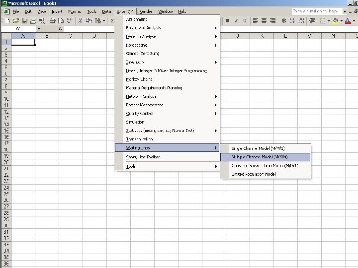


Template and Sample Data
 machines which are repaired")
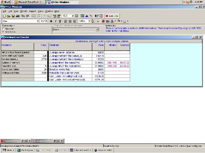
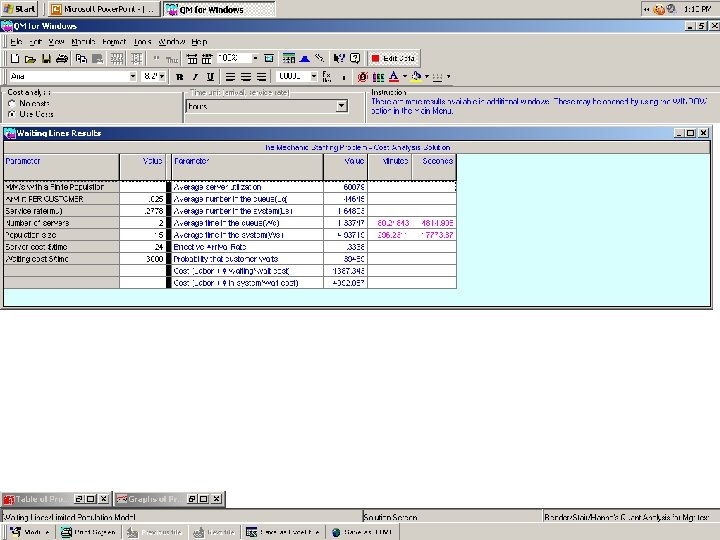
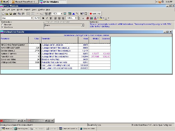
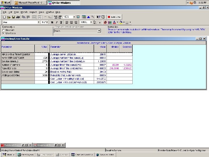
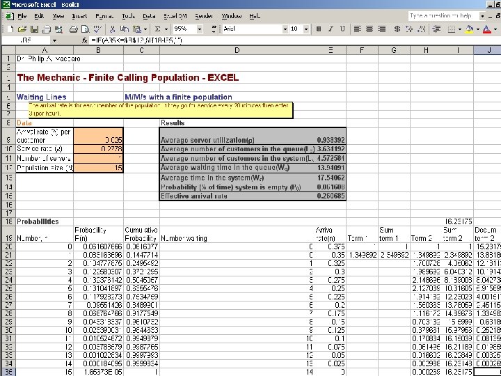
Finite Calling Population Model Application A shop has fifteen (15) machines which are repaired in the same order in which they fail. The machines fail according to a poisson distribution, and the service times are exponentially distributed. One (1) mechanic is on-duty. A machine fails on average, every forty (40) hours. The average repair takes 3. 6 hours. N = 15 machines λ = 1/40 th of a machine per hour =. 0250 machine per hour μ = 1/3. 6 th of a machine per hour =. 2778 machine per hour

Finite Calling Population Model Probability that the system is empty: Po = 1 N Σ n=0 N! (N – n)! λ μ n N = size of the finite calling population

Finite Calling Population Model Average length of the queue Lq = N – λ + μ λ ( 1 – Po )
 in the system: L =")
Finite Calling Population Model Average number of customers (items) in the system: L = Lq + ( 1 – Po ) Average waiting time in the queue: Wq = Lq (N–L)λ Average time in the system: W = Wq + ( 1 / μ )

Finite Calling Population Model Application 1 Po = 15 Σ n=0 Lq = 15 – 15! ( 15 – n )! . 0250 +. 2778. 0250. 2778 n =. 0616 = 6. 16% ( 1 -. 0616 ) = 3. 63 machines

Finite Calling Population Model APPLICATION L = 3. 63 + ( 1 -. 0616 ) = 4. 57 machines Wq = 3. 63 = 13. 94 hours ( 15 – 4. 57 ) (. 0250 ) W = 13. 94 + ( 1 /. 2778 ) = 17. 54 hours

Finite Calling Population Model Performance Summary Number of Mechanics M=1 M=2 M=3 M=4 Utilization Rate (ρ) Average Wait Line (Lq) Average Number In System (L) Average Wait (Wq) Average Time In System (W) Probability of Waiting (Pw) . 9384 3. 63 Machines 4. 57 Machines 13. 94 Hours 17. 54 Hours 91. 14% . 6008 . 4464 Machines 1. 648 Machines 1. 337 Hours 4. 9372 Hours 39. 49% . 4109 . 0678 Machines 1. 300 Machines . 198 Hours 3. 7977 Hours 11. 47% . 3094 . 0099 Machines 1. 247 Machines . 0287 Hours 3. 6284 Hours . 0251

Finite Calling Population Model Cost Summary Number of Mechanics Total Hourly Wage Average Number In System (L) Total Hourly Opportunity Cost Total Cost M=1 $24. 00 4. 57 Machines $13, 710. 00 $13, 734. 00 M=2 $48. 00 1. 648 Machines 4, 944. 00 $4, 992. 00 M=3 $72. 00 1. 300 Machines $3, 900. 00 $3, 972. 00 M=4 $96. 00 1. 247 Machines $3, 741. 00 $3, 837. 00 Assume Machine Hourly Opportunity Cost of $3, 000. 00

QM for Windows QUEUING APPLICATIONS The Mechanic Problem operational analysis and cost analysis Single-Channel Single-Phase Finite Calling Population Model

We assume that a mechanic earns $24. 00 per hour on average. We also assume that the opportunity cost of an out-of-service machine is $3, 000. 00 per hour.


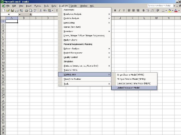
Queuing Theory Modeling with Single-Channel Single-Phase Finite Calling Population Model The Mechanic Problem ( operational analysis only )


Template and Sample Data

Kendall-Lee Convention v Widely accepted classification system for queuing models. v Indicates the pattern of arrivals, the service time distribution, and the number of channels in a model. v Often encountered in queuing software. v Known also as the Kendall Notation.

Basic Three - Symbol Notation The Template Arrival Distribution 1 st Where: Service Time Distribution 2 nd Service Channels Open 3 rd M = poisson distribution D = constant (deterministic) rate G = general distribution with mean and variance known m / s = number of channels or servers

1 st Example M Poisson Arrival Distribution M Negative Exponential Service Time Distribution 1 SINGLE-CHANNEL SINGLE-SERVER MODEL

2 nd Example M Poisson Arrival Distribution M Negative Exponential Service Time Distribution m MULTI-CHANNEL MULTI-SERVER MODEL

2 nd Example M Poisson Arrival Distribution M Negative Exponential Service Time Distribution s MULTI-CHANNEL MULTI-SERVER MODEL

3 rd Example M M WITH FINITE POPULATION Poisson Arrival Distribution Negative Exponential Service Time Distribution 1 Imposed Legend SINGLE-CHANNEL SINGLE-SERVER MODEL WITH FINITE CALLING POPULATION

4 th Example M Poisson Arrival Distribution D Constant Service Time Distribution 3 TRIPLE-CHANNEL TRIPLE-SERVER MODEL

MD 3 Example q 3 stamping machines in a work center q 5 second fixed stamp time per inserted disc q blank steel discs follow a poisson arrival pattern into the center

5 th Example M Poisson Arrival Distribution G The Normal Curve Service Time Distribution 2 DUAL-CHANNEL DUAL-SERVER MODEL

MG 2 Example μ = 2. 0 min σ = 30 secs M=2 q An office copy room has 2 copiers q Copy job time is normally distributed q The mean copy job time is 2 minutes q The standard deviation is 30 seconds q Employees follow a poisson arrival pattern into the copy room

What We Have Seen PROBLEM The Convenience Store Clerk The Loan Officers The Mechanic MODEL M/M/1 M/M/m or M/M/s M / 1 with finite calling population

QUEUING THEORY Applied Management Science for Decision Making, 1 e © 2012 Pearson Prentice-Hall, Inc. Philip A. Vaccaro , Ph. D

Solved Problems Queuing Theory Computer-Based Manual Applied Management Science for Decision Making, 1 e © 2010 Pearson Prentice-Hall, Inc. Philip A. Vaccaro , Ph. D

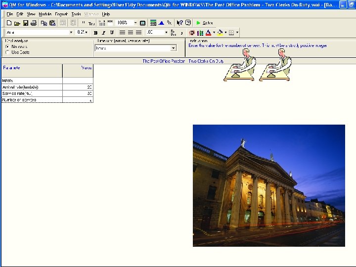
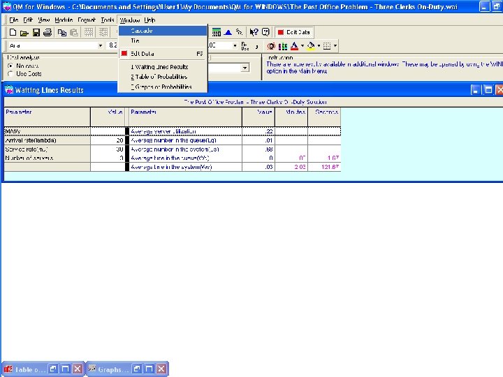
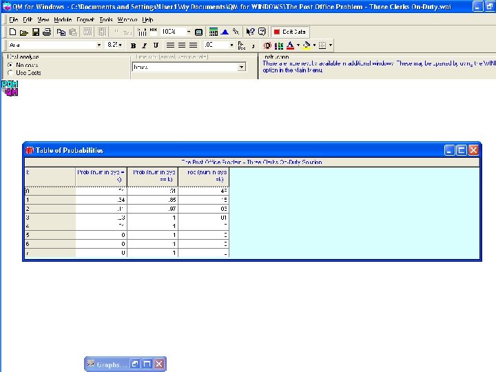
The Post Office Queuing Theory Problem 1 A post office has a single line for customers to use while waiting for the next available postal clerk. There are two postal clerks who work at the same rate. The arrival rate of customers follows a poisson distribution, while the service time follows an exponential distribution. The average arrival rate is one customer every three ( 3 ) minutes and the average service rate is one customer every two ( 2 ) minutes for each of the two clerks. The facility is idle 50% of the time ( Po =. 50 ).

The Post Office Queuing Theory REQUIREMENT: 1. What is the average length of the line? 2. How long does the average person spend waiting for a clerk to become available? 3. What proportion of the time are both clerks idle? Po =. 50 BUT NOW SHOW ALL SUPPORTING CALCULATIONS

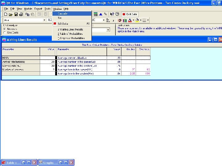
The Post Office Queuing Theory Problem 1 Given: λ = 20 and μ = 30 ( per hour rates ) and M = 2 The average number of customers in the system ( L ) ( 20 x 30 ) (. 67 ) ( 2 - 1 )! (2 x 30 – 20) 600 (. 4489 ) L= ( 60 – 20 ) 2 Po =. 50 2 L= *: 2 x (. 50 ) +. 67 X (. 50 ) +. 67 =. 754165 * L needs to be calculated before Lq can be found.

The Post Office Queuing Theory Problem 1 Given: λ = 20 and μ = 30 ( per hour rates ) and M = 2 The average length of the line ( Lq ) : Lq = L – ( λ / μ ) Lq =. 7541 – ( 20 / 30 ) =. 0841

The Post Office Queuing Theory REQUIREMENT: 1. What is the average length of the line? 2. How long does the average person spend waiting for a clerk to become available? 3. What proportion of the time are both clerks idle? Po =. 50 BUT NOW SHOW ALL SUPPORTING CALCULATIONS

The Post Office Queuing Theory Problem 1 The average time in the system ( W ) : W = L / λ = (. 7541 / 20 ) =. 0377 of an hour or 2. 25 minutes The average time in the queue ( Wq ) : Wq = Lq / λ = (. 0841 / 20 ) =. 0042 of an hour or. 25 minutes

The Post Office Queuing Theory REQUIREMENT: 1. What is the average length of the line? 2. How long does the average person spend waiting for a clerk to become available? 3. What proportion of the time are both clerks idle? Po =. 50 BUT NOW SHOW ALL SUPPORTING CALCULATIONS

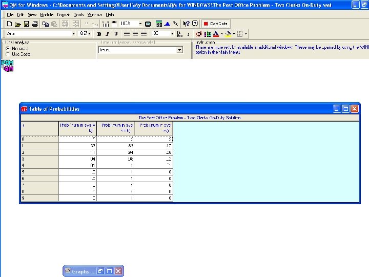
The Post Office Queuing Theory 1 Po = 1 20 0 1 20 + 0! 30 1! 30 2 1 1 + (2)(1) x 20 x 30 2(30) - 20 1 Po = [ 1 +. 67 ] +. 50 (. 4489 ) ( 1. 5 ) Po =. 50 - THE PROBABILITY THAT THE POST OFFICE IS IDLE

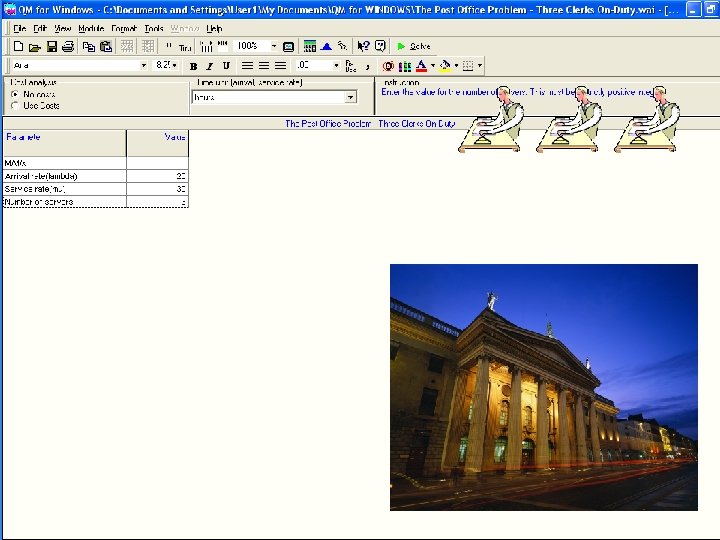
The Post Office Revisited Queuing Theory Problem 2 A post office has a single line for customers to use while waiting for the next available postal clerk. There are three postal clerks who work at the same rate. The arrival rate of customers follows a poisson distribution, while the service time follows an exponential distribution. The average arrival rate is one customer every three ( 3 ) minutes and the average service rate is one customer every two minutes for each of the three clerks. The facility is idle 51. 22% of the time ( Po =. 5122 ).

The Post Office Revisited Queuing Theory REQUIREMENT: 1. What is the average length of the line? 2. How long does the average person spend waiting for a clerk to become available? 3. What proportion of the time are all three clerks idle? Po =. 5122 BUT NOW SHOW ALL SUPPORTING CALCULATIONS

The Post Office Revisted Queuing Theory Problem 2 Given: λ = 20 and μ = 30 ( per hour rates ) and M = 3 The average number of customers in the system ( L ) ( 20 x 30 ) (. 67 ) 3 L= ( 3 - 1 )! (3 x 30 – 20) 600 (. 300763 ) L= 2! ( 90 – 20 ) 2 *: 2 x (. 5122 ) +. 67 X Po =. 5122 Given (. 5122 ) +. 67 =. 6794 * L needs to be calculated before Lq can be found.

The Post Office Revisited Queuing Theory Problem 2 Given: λ = 20 and μ = 30 ( per hour rates ) and M = 3 The average length of the line ( Lq ) : Lq = L – ( λ / μ ) Lq =. 6794 – ( 20 / 30 ) =. 0094

The Post Office Revisted Queuing Theory REQUIREMENT: 1. What is the average length of the line? 2. How long does the average person spend waiting for a clerk to become available? 3. What proportion of the time are all three clerks idle? Po =. 5122 BUT NOW SHOW ALL SUPPORTING CALCULATIONS

The Post Office Revisited Queuing Theory Problem 2 The average time in the system ( W ) : W = L / λ = (. 6794 / 20 ) =. 0339 of an hour or 2. 028 minutes The average time in the queue ( Wq ) : Wq = Lq / λ = (. 0094 / 20 ) =. 00047 of an hour or. 028 minutes

The Post Office Revisited Queuing Theory REQUIREMENT: 1. What is the average length of the line? 2. How long does the average person spend waiting for a clerk to become available? 3. What proportion of the time are all three clerks idle? Po =. 5122 BUT NOW SHOW ALL SUPPORTING CALCULATIONS

The Post Office Revisited Queuing Theory 1 Po = 0 1 20 0! 30 + 1 1 20 1! 30 3 2 1 + 20 2! 30 1 + (3)(2)(1) x 20 30 x 3(30) - 20 1 Po = [ 1 +. 67 +. 2244 ] +. 166 (. 3007 ) ( 1. 285 ) Po ≈. 5122 THE PROBABILITY THAT THE POST OFFICE IS IDLE

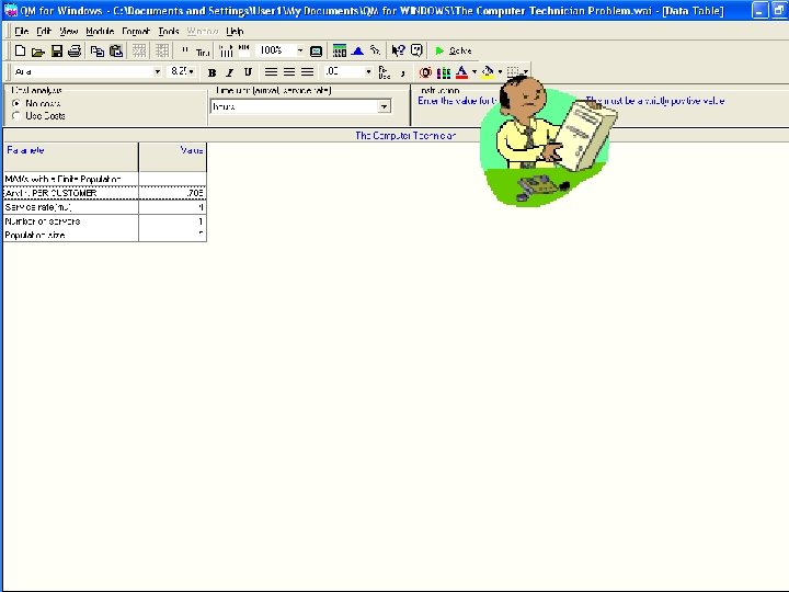
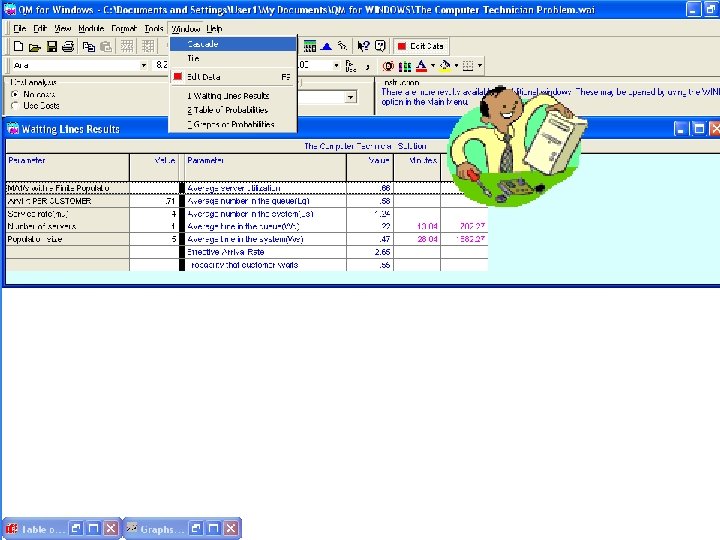
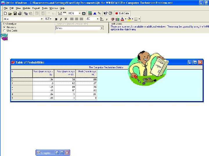
The Computer Technician Queuing Theory Problem 3 A technician monitors a group of five (5) computers that run an automated manufacturing facility. It takes an average of fifteen (15) minutes ( exponentially distributed ) to adjust a computer that developes a problem. The computers run for an average of eighty-five (85) minutes ( poisson distributed ) without requiring adjustments.

The Computer Technician Queuing Theory Problem 3 REQUIREMENT : 1. 2. 3. 4. 5. What is the average number of computers waiting for adjustment? What is the average number of computers not in working order? What is the probability that the system is empty? What is the average time in the queue? What is the average time in the system? Note: Po =. 344 or 34. 4% ( no need to manually compute! )

The Computer Technician Queuing Theory Problem 3 Given: λ = 60/85 =. 706 computers ; μ = 4 computers ; N = 5 M = 1 ( technician ) ; Po =. 344 Average number of computers waiting for adjustment : Lq = N - λ+μ (1 – Po ) λ Lq = 5 – 4. 706 (. 66 ) = 5 – 4. 4 =. 576

The Computer Technician Queuing Theory Problem 3 REQUIREMENT : 1. 2. 3. 4. 5. What is the average number of computers waiting for adjustment? What is the average number of computers not in working order? What is the probability that the system is empty? What is the average time in the queue? What is the average time in the system? Note: Po =. 344 or 34. 4% ( no need to manually compute! )

The Computer Technician Queuing Theory Problem 3 The average number of computers not in working order: L = Lq + ( 1 – Po ) L =. 576 + ( 1 -. 34 ) = 1. 24

The Computer Technician Queuing Theory Problem 3 REQUIREMENT : 1. 2. 3. 4. 5. What is the average number of computers waiting for adjustment? What is the average number of computers not in working order? What is the probability that the system is empty? What is the average time in the queue? What is the average time in the system? Note: Po =. 344 or 34. 4% ( no need to manually compute! )

The Computer Technician Queuing Theory Problem 3 The probability that the system is empty : Po = 0. 344 ( as given )

The Computer Technician Queuing Theory Problem 3 REQUIREMENT : 1. 2. 3. 4. 5. What is the average number of computers waiting for adjustment? What is the average number of computers not in working order? What is the probability that the system is empty? What is the average time in the queue? What is the average time in the system? Note: Po =. 344 or 34. 4% ( no need to manually compute! )

The Computer Technician Queuing Theory Problem 3 The average time in the queue : Lq Wq = (N–L)λ. 576 ( 5 – 1. 24 )(. 706 ) =. 217 of an hour

The Computer Technician Queuing Theory Problem 3 REQUIREMENT : 1. 2. 3. 4. 5. What is the average number of computers waiting for adjustment? What is the average number of computers not in working order? What is the probability that the system is empty? What is the average time in the queue? What is the average time in the system? Note: Po =. 344 or 34. 4% ( no need to manually compute! )

The Computer Technician Queuing Theory Problem 3 The average time in the system : W = Wq + (1/μ) W =. 217 + ( 1 / 4 ) =. 217 +. 25 =. 467 of an hour

Solved Problems Queuing Theory Computer-Based Manual Applied Management Science for Decision Making, 1 e © 2010 Pearson Prentice-Hall, Inc. Philip A. Vaccaro , Ph. D
b612ee9767285f6e07b4797e116e6156.ppt