b25694d92a4bdc7185ac7b42db5e4f2e.ppt
- Количество слайдов: 24
 Queuing Theory Jackson Networks
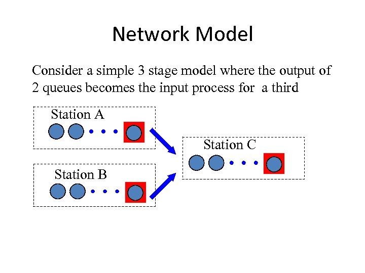 Network Model Consider a simple 3 stage model where the output of 2 queues becomes the input process for a third Station A Station C Station B
 Network Model Station A Station C Station B Proposition 1: rate in = rate out, that is, if l. A and l. B are the input rates for station A and B respectively, then the input rate for station C is l. A+l. B. Proposition 2: exponential inter-arrivals at A and B provide exponential inter-arrivals at station C.
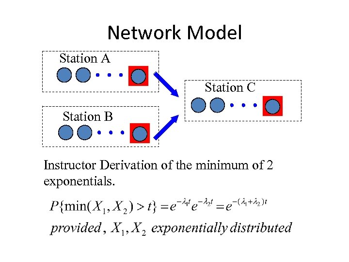 Network Model Station A Station C Station B Instructor Derivation of the minimum of 2 exponentials.
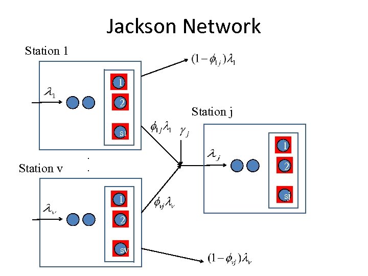 Jackson Network Station 1 1 2 Station j s 1 Station v 1 . . 2 1 2 sv sj
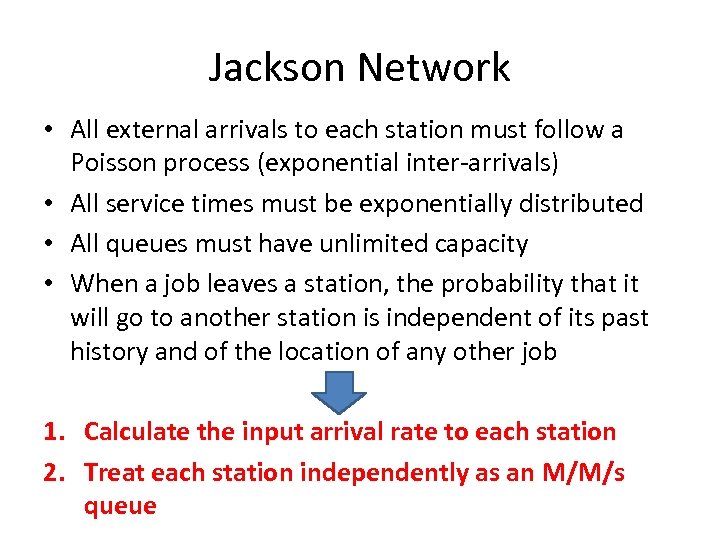 Jackson Network • All external arrivals to each station must follow a Poisson process (exponential inter-arrivals) • All service times must be exponentially distributed • All queues must have unlimited capacity • When a job leaves a station, the probability that it will go to another station is independent of its past history and of the location of any other job 1. Calculate the input arrival rate to each station 2. Treat each station independently as an M/M/s queue
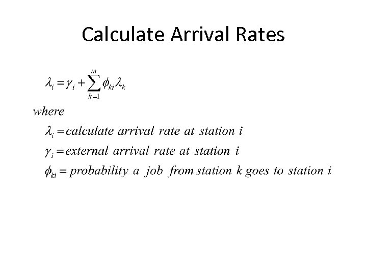 Calculate Arrival Rates
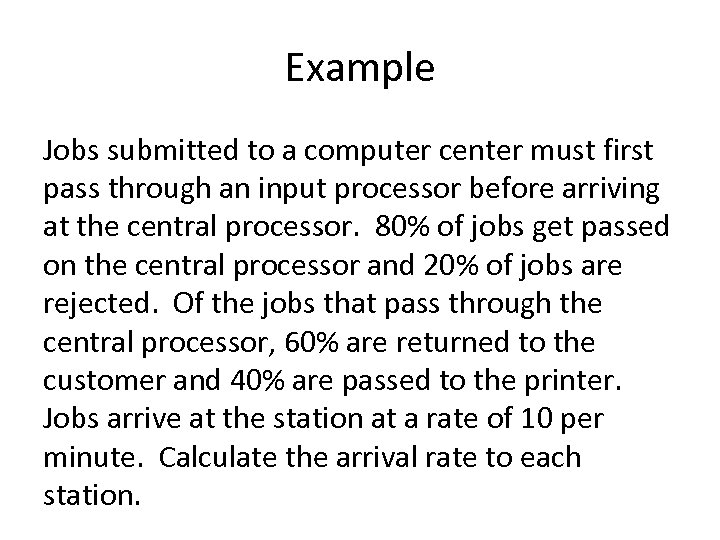 Example Jobs submitted to a computer center must first pass through an input processor before arriving at the central processor. 80% of jobs get passed on the central processor and 20% of jobs are rejected. Of the jobs that pass through the central processor, 60% are returned to the customer and 40% are passed to the printer. Jobs arrive at the station at a rate of 10 per minute. Calculate the arrival rate to each station.
 Example. 6 . 2 10 Input . 8 Central . 4 Printer
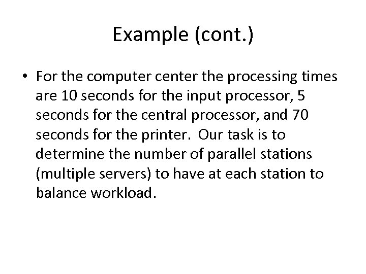 Example (cont. ) • For the computer center the processing times are 10 seconds for the input processor, 5 seconds for the central processor, and 70 seconds for the printer. Our task is to determine the number of parallel stations (multiple servers) to have at each station to balance workload.
 Example 10 Input 8 Central 3. 2 Printer For our initial try, we will solve for s 1 = 2, s 2 = 1, s 3 = 4
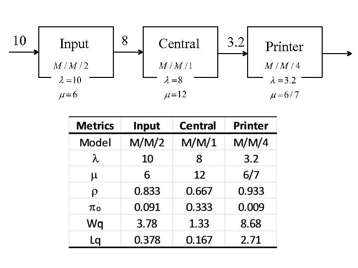 10 Input 8 Central 3. 2 Printer
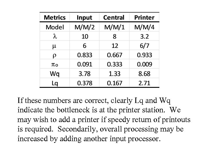 If these numbers are correct, clearly Lq and Wq indicate the bottleneck is at the printer station. We may wish to add a printer if speedy return of printouts is required. Secondarily, overall processing may be increased by adding another input processor.
 Job Shop Example • An electronics firm has 3 different products in a job shop environment. The job shop has six different machines with multiple machines at 5 of the 6 stations. Product Order rate Flow 1 30/month ABDF 2 10/month ABEF 3 20/month ACEF Summary information is on the network below.
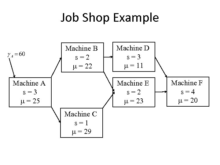 Job Shop Example Machine B s=2 m = 22 Machine A s=3 m = 25 Machine D s=3 m = 11 Machine E s=2 m = 23 Machine C s=1 m = 29 Machine F s=4 m = 20
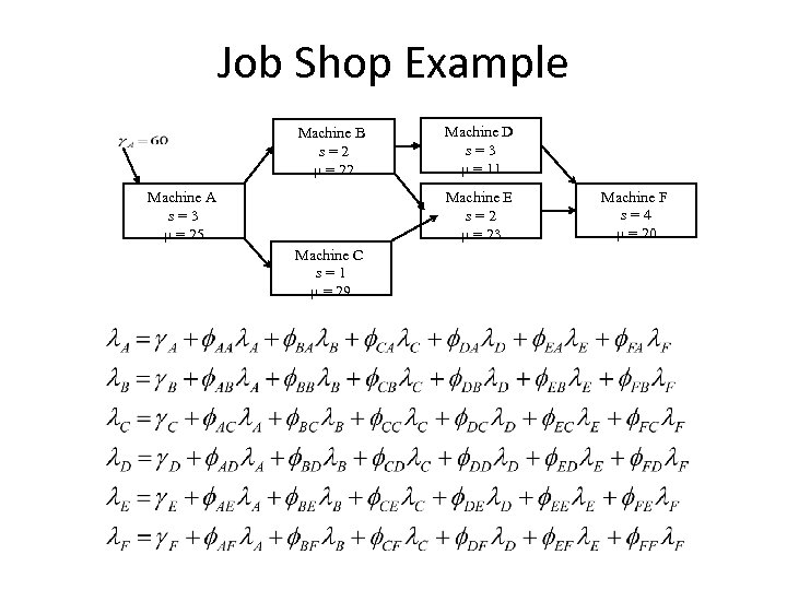 Job Shop Example Machine B s=2 m = 22 Machine A s=3 m = 25 Machine D s=3 m = 11 Machine E s=2 m = 23 Machine C s=1 m = 29 Machine F s=4 m = 20
 Job Shop Example Machine B s=2 m = 22 Machine A s=3 m = 25 Machine D s=3 m = 11 Machine E s=2 m = 23 Machine C s=1 m = 29 Machine F s=4 m = 20
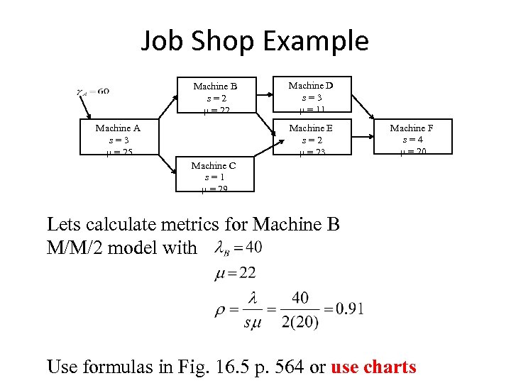 Job Shop Example Machine B s=2 m = 22 Machine A s=3 m = 25 Machine D s=3 m = 11 Machine E s=2 m = 23 Machine F s=4 m = 20 Machine C s=1 m = 29 Lets calculate metrics for Machine B M/M/2 model with Use formulas in Fig. 16. 5 p. 564 or use charts
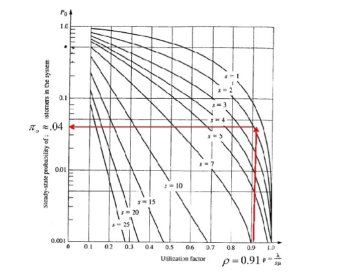

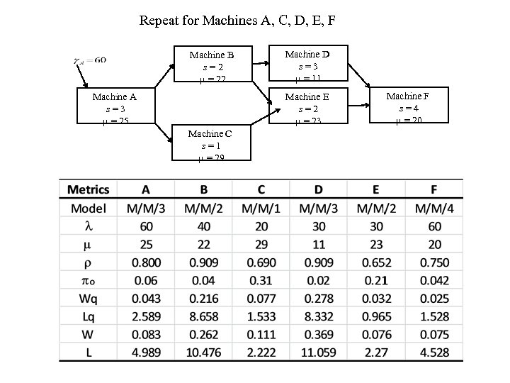 Repeat for Machines A, C, D, E, F Machine B s=2 m = 22 Machine A s=3 m = 25 Machine D s=3 m = 11 Machine E s=2 m = 23 Machine C s=1 m = 29 Machine F s=4 m = 20
 Interesting Application to Manufacturing Note that lead time is just the time in the system which for product 1 which has sequence ABDF is W = total time in system = lead time = WA + WB + WD + WF =. 789 WIP = work in process = parts per month x lead time = 30(. 789) = 23. 67
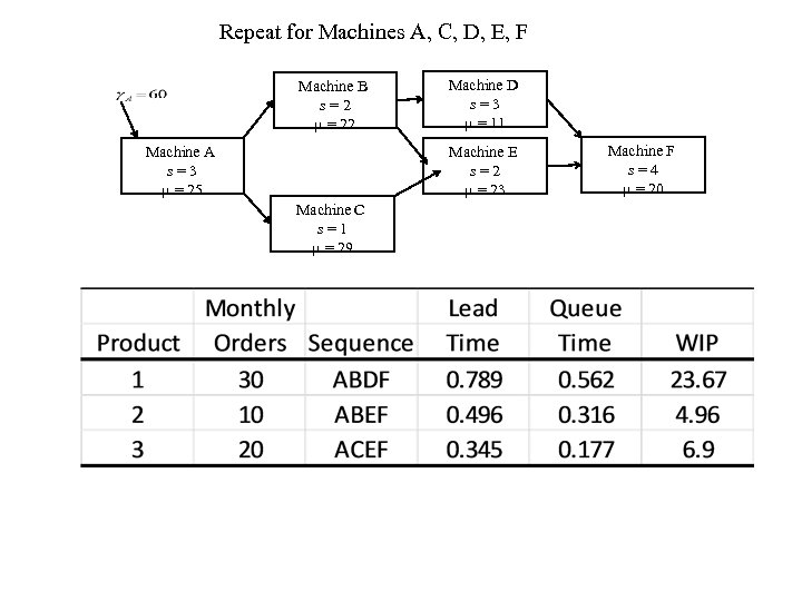 Repeat for Machines A, C, D, E, F Machine B s=2 m = 22 Machine A s=3 m = 25 Machine D s=3 m = 11 Machine E s=2 m = 23 Machine C s=1 m = 29 Machine F s=4 m = 20
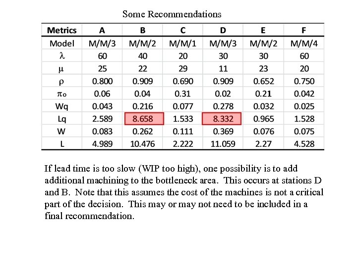 Some Recommendations If lead time is too slow (WIP too high), one possibility is to additional machining to the bottleneck area. This occurs at stations D and B. Note that this assumes the cost of the machines is not a critical part of the decision. This may or may not need to be included in a final recommendation.


