Queuing Systems Chapter 17 Chapter Topics

Queuing Systems Chapter 17

Chapter Topics § Elements of Waiting Line Analysis § Single-Server Waiting Line System § Undefined and Constant Service Times § Finite Queue Length § Finite Calling Problem § Multiple-Server Waiting Line § Addition Types of Queuing Systems

Overview § People and products spent significant amount of time in waiting lines § Providing quick service is an important aspect of customer service § Trade-off between the cost of improving service and the costs associated with making customers wait § A probabilistic form of analysis § Results are referred to as operating characteristics § Results are used to make decisions

Elements of Waiting Line Analysis § Waiting lines form because people arrive at a service faster than they can be served § Not arrive at a constant rate nor are they served in an equal amount of time § Have an average rate of customer arrivals and an average service time § Decisions are based on these averages for customer arrivals and service times § Formulas are used to compute operating characteristics

Single-Server Waiting Line System § Components include: § Arrivals (customers), servers, (cash register/operator), customers in line form a waiting line § Factors to consider: § queue discipline. § nature of the calling population § arrival rate § service rate.

Component Definitions § Queue Discipline: order in which customers are served (FIFO, LIFO, or randomly) § Calling Population: source of customers (infinite or finite) § Arrival Rate: Frequency at which customers arrive at a waiting line according to a probability distribution (Poisson distribution) § Service Rate: Average number of customers that can be served during a time period (negative exponential distribution)

Single-Server Waiting Line System Single-Server Model § Assumptions: § An infinite calling population § A first-come, first-served queue discipline § Poisson arrival rate § Exponential service times § Symbology: § = the arrival rate (average number of arrivals/time period) § = the service rate (average number served/time period) § Customers must be served faster than they arrive ( < )

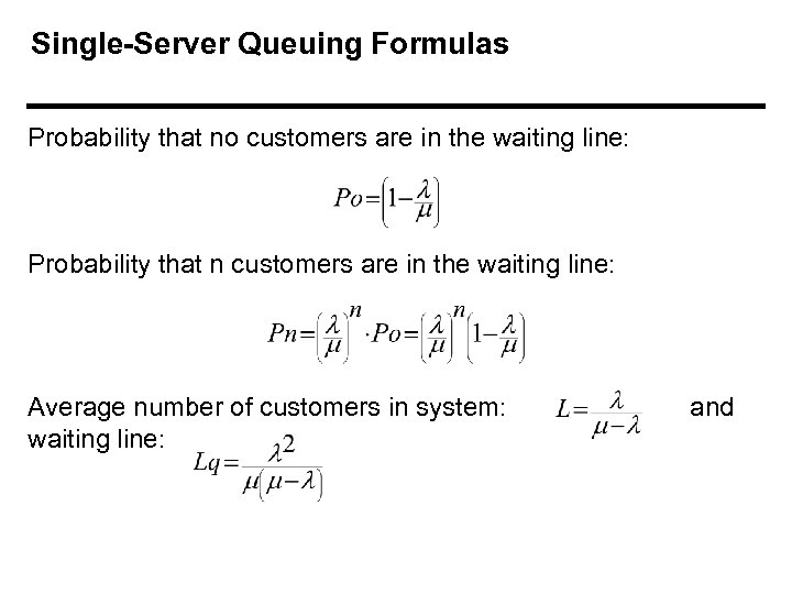Single-Server Queuing Formulas Probability that no customers are in the waiting line: Probability that n customers are in the waiting line: Average number of customers in system: waiting line: and

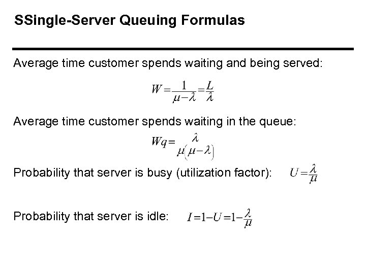SSingle-Server Queuing Formulas Average time customer spends waiting and being served: Average time customer spends waiting in the queue: Probability that server is busy (utilization factor): Probability that server is idle:

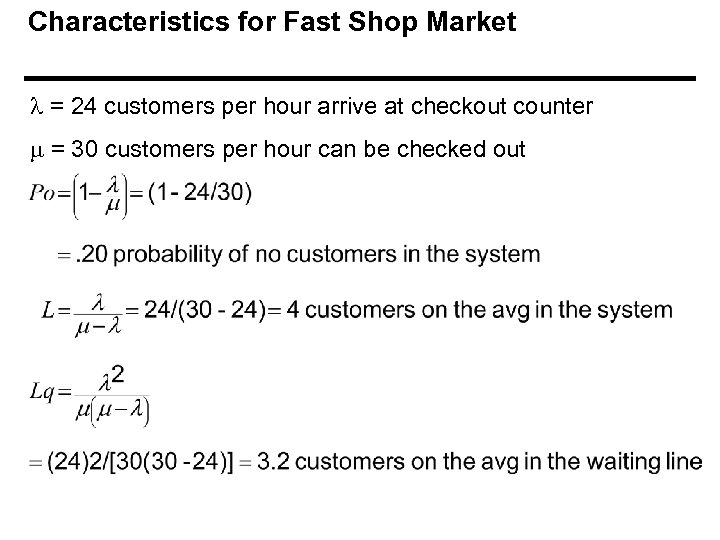Characteristics for Fast Shop Market = 24 customers per hour arrive at checkout counter = 30 customers per hour can be checked out

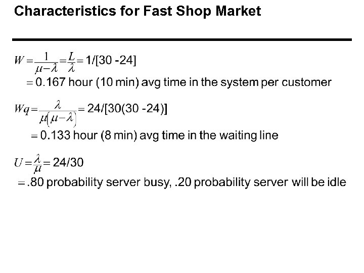Characteristics for Fast Shop Market

Steady-State Operating Characteristics § Utilization factor, U, must be less than one: § U < 1, or / < 1 and < . § Ratio of the arrival rate to the service rate must be less than one or, the service rate must be greater than the arrival rate § Server must be able to serve customers faster than the arrival rate in the long run, or waiting line will grow to infinite size.

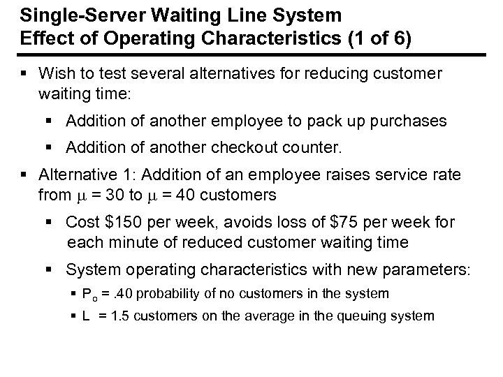Single-Server Waiting Line System Effect of Operating Characteristics (1 of 6) § Wish to test several alternatives for reducing customer waiting time: § Addition of another employee to pack up purchases § Addition of another checkout counter. § Alternative 1: Addition of an employee raises service rate from = 30 to = 40 customers § Cost $150 per week, avoids loss of $75 per week for each minute of reduced customer waiting time § System operating characteristics with new parameters: § Po =. 40 probability of no customers in the system § L = 1. 5 customers on the average in the queuing system

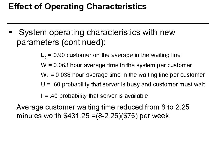Effect of Operating Characteristics § System operating characteristics with new parameters (continued): Lq = 0. 90 customer on the average in the waiting line W = 0. 063 hour average time in the system per customer Wq = 0. 038 hour average time in the waiting line per customer U =. 60 probability that server is busy and customer must wait I =. 40 probability that server is available Average customer waiting time reduced from 8 to 2. 25 minutes worth $431. 25 =(8 -2. 25)($75) per week.

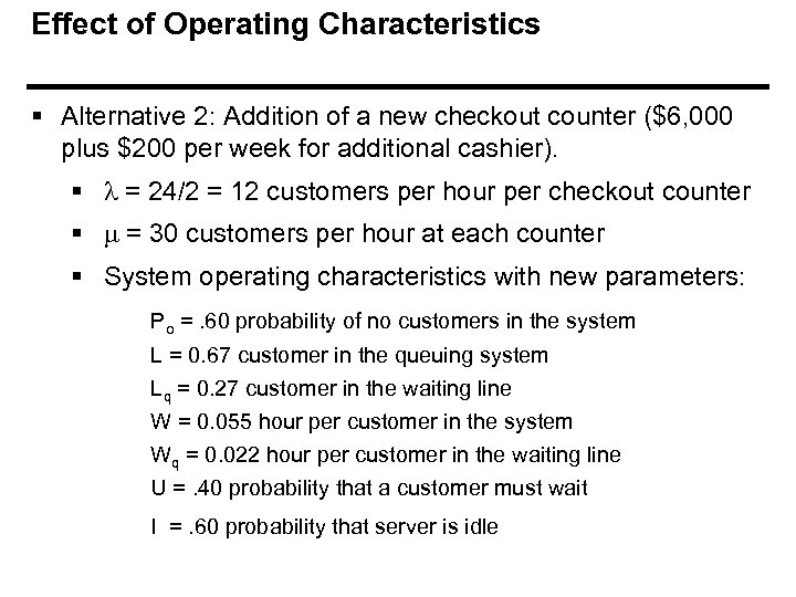Effect of Operating Characteristics § Alternative 2: Addition of a new checkout counter ($6, 000 plus $200 per week for additional cashier). § = 24/2 = 12 customers per hour per checkout counter § = 30 customers per hour at each counter § System operating characteristics with new parameters: Po =. 60 probability of no customers in the system L = 0. 67 customer in the queuing system Lq = 0. 27 customer in the waiting line W = 0. 055 hour per customer in the system Wq = 0. 022 hour per customer in the waiting line U =. 40 probability that a customer must wait I =. 60 probability that server is idle

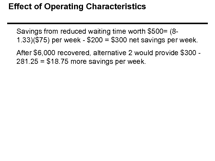Effect of Operating Characteristics Savings from reduced waiting time worth $500= (81. 33)($75) per week - $200 = $300 net savings per week. After $6, 000 recovered, alternative 2 would provide $300 281. 25 = $18. 75 more savings per week.

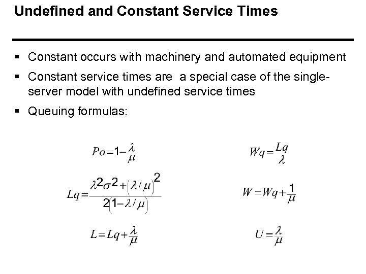Undefined and Constant Service Times § Constant occurs with machinery and automated equipment § Constant service times are a special case of the singleserver model with undefined service times § Queuing formulas:

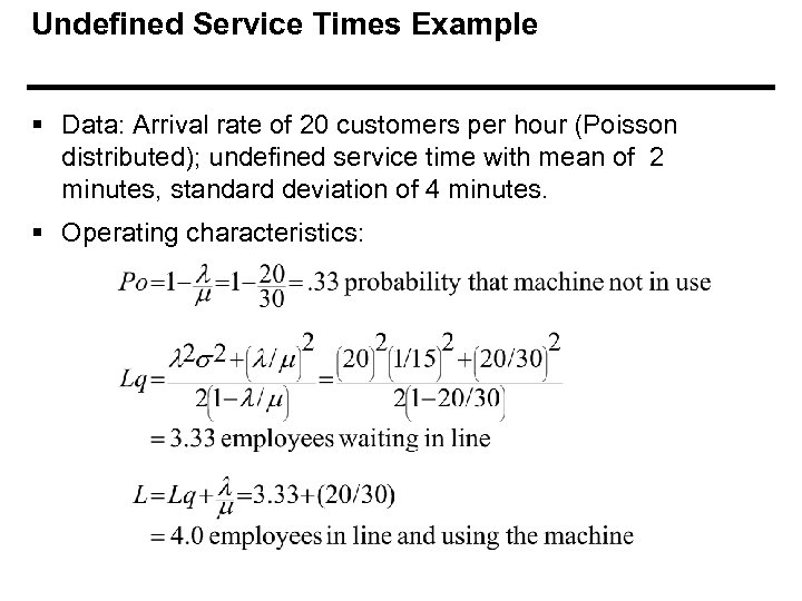Undefined Service Times Example § Data: Arrival rate of 20 customers per hour (Poisson distributed); undefined service time with mean of 2 minutes, standard deviation of 4 minutes. § Operating characteristics:

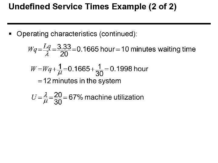Undefined Service Times Example (2 of 2) § Operating characteristics (continued):

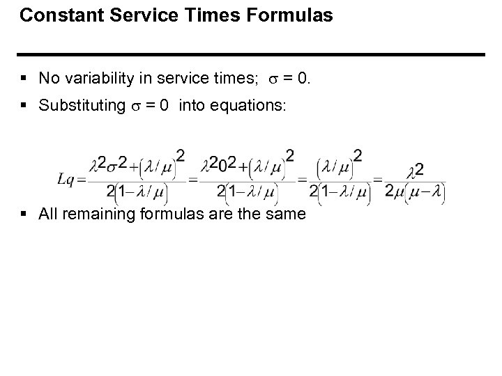Constant Service Times Formulas § No variability in service times; = 0. § Substituting = 0 into equations: § All remaining formulas are the same

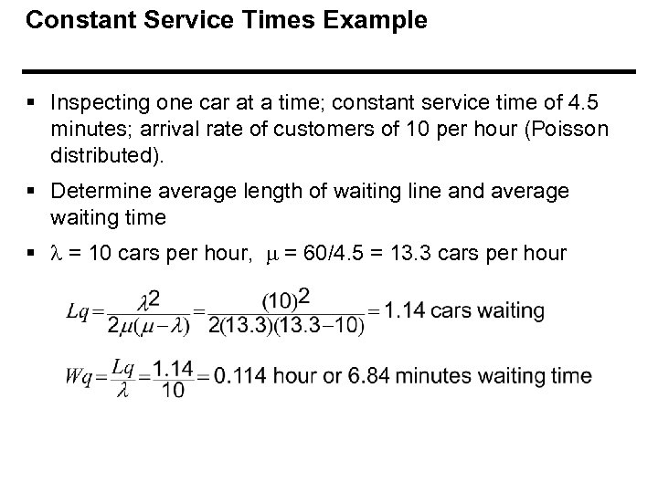Constant Service Times Example § Inspecting one car at a time; constant service time of 4. 5 minutes; arrival rate of customers of 10 per hour (Poisson distributed). § Determine average length of waiting line and average waiting time § = 10 cars per hour, = 60/4. 5 = 13. 3 cars per hour

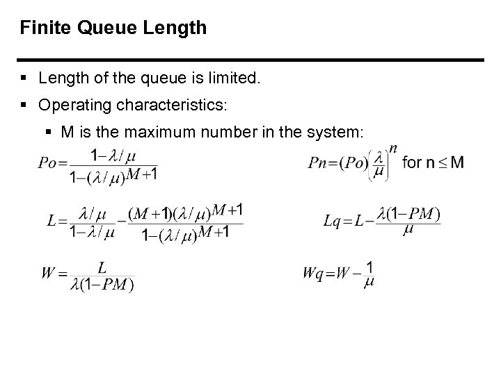Finite Queue Length § Length of the queue is limited. § Operating characteristics: § M is the maximum number in the system:

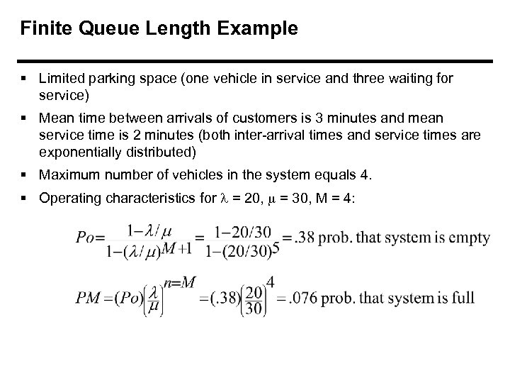Finite Queue Length Example § Limited parking space (one vehicle in service and three waiting for service) § Mean time between arrivals of customers is 3 minutes and mean service time is 2 minutes (both inter-arrival times and service times are exponentially distributed) § Maximum number of vehicles in the system equals 4. § Operating characteristics for = 20, = 30, M = 4:

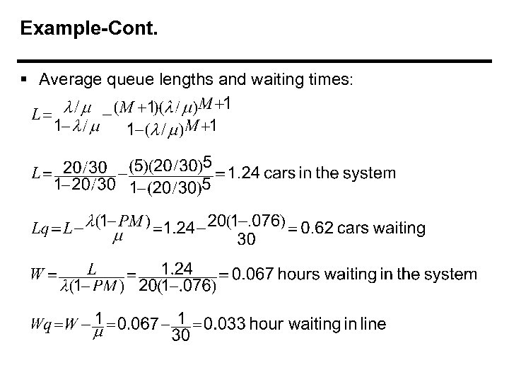Example-Cont. § Average queue lengths and waiting times:

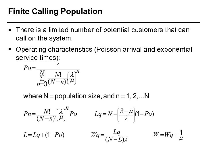Finite Calling Population § There is a limited number of potential customers that can call on the system. § Operating characteristics (Poisson arrival and exponential service times):

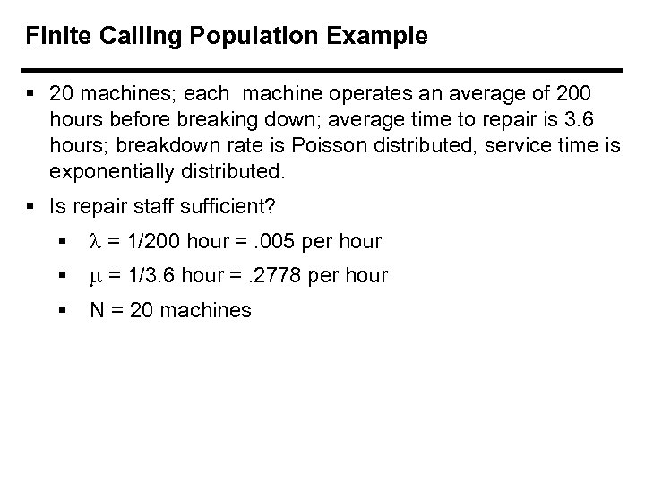Finite Calling Population Example § 20 machines; each machine operates an average of 200 hours before breaking down; average time to repair is 3. 6 hours; breakdown rate is Poisson distributed, service time is exponentially distributed. § Is repair staff sufficient? § = 1/200 hour =. 005 per hour § = 1/3. 6 hour =. 2778 per hour § N = 20 machines

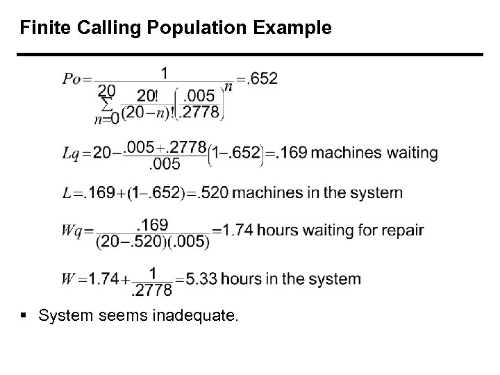Finite Calling Population Example § System seems inadequate.

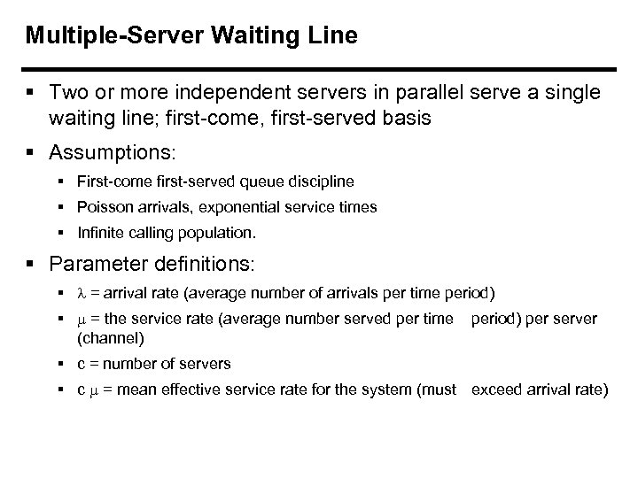Multiple-Server Waiting Line § Two or more independent servers in parallel serve a single waiting line; first-come, first-served basis § Assumptions: § First-come first-served queue discipline § Poisson arrivals, exponential service times § Infinite calling population. § Parameter definitions: § = arrival rate (average number of arrivals per time period) § = the service rate (average number served per time (channel) period) per server § c = number of servers § c = mean effective service rate for the system (must exceed arrival rate)

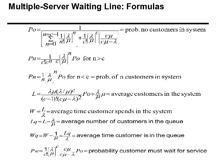Multiple-Server Waiting Line: Formulas

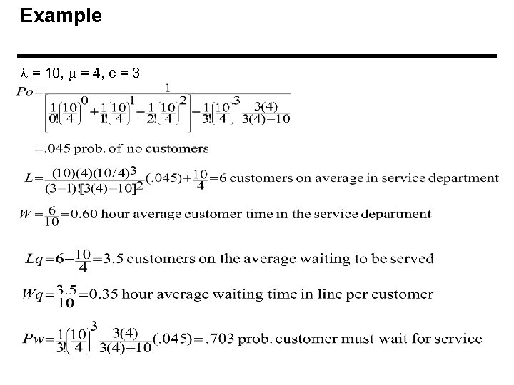Example = 10, = 4, c = 3

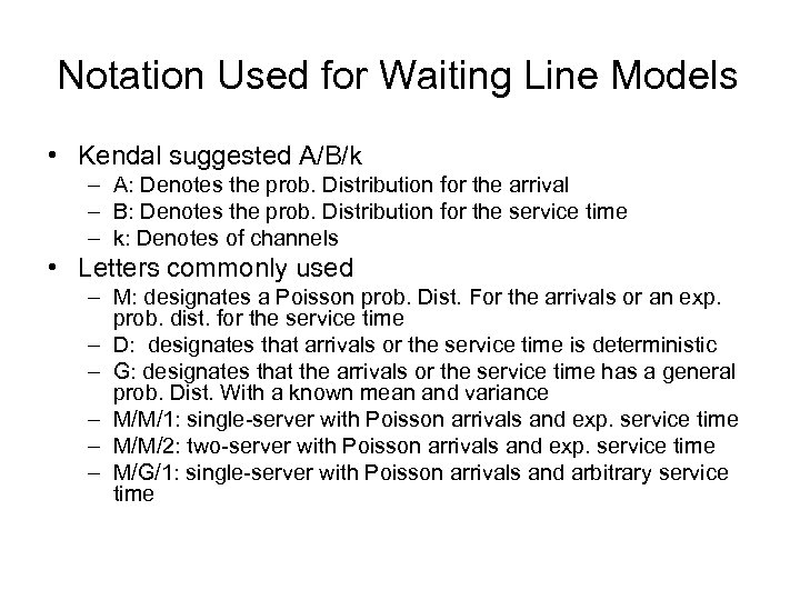Notation Used for Waiting Line Models • Kendal suggested A/B/k – A: Denotes the prob. Distribution for the arrival – B: Denotes the prob. Distribution for the service time – k: Denotes of channels • Letters commonly used – M: designates a Poisson prob. Dist. For the arrivals or an exp. prob. dist. for the service time – D: designates that arrivals or the service time is deterministic – G: designates that the arrivals or the service time has a general prob. Dist. With a known mean and variance – M/M/1: single-server with Poisson arrivals and exp. service time – M/M/2: two-server with Poisson arrivals and exp. service time – M/G/1: single-server with Poisson arrivals and arbitrary service time

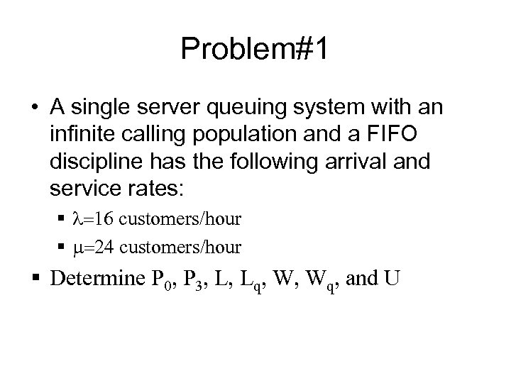Problem#1 • A single server queuing system with an infinite calling population and a FIFO discipline has the following arrival and service rates: § =16 customers/hour § =24 customers/hour § Determine P 0, P 3, L, Lq, W, Wq, and U