Queues in Hospitals Semi-Open Queueing Networks in the

Queues in Hospitals: Semi-Open Queueing Networks in the QED Regime Galit Yom-Tov Joint work with Avishai Mandelbaum Technion – Israel Institute of Technology 31/Dec/2008

Agenda Introduction n Medical Unit Model n Mathematical Results n Numerical Example n Time-varying Model n Future Research n 2

Work-Force and Bed Capacity Planning n n n Total health expenditure as percentage of gross domestic product: Israel 8%, EU 10%, USA 14%. Human resource constitute 70% of hospital expenditure. There are 3 M registered nurses in the U. S. but still a chronic shortage. California law set nurse-to-patient ratios such as 1: 6 for pediatric care unit. O. B. Jennings and F. de Véricourt (2008) showed that fixed ratios do not account for economies of scale. Management measures average occupancy levels, while arrivals have seasonal patterns and stochastic 3 variability (Green 2004).

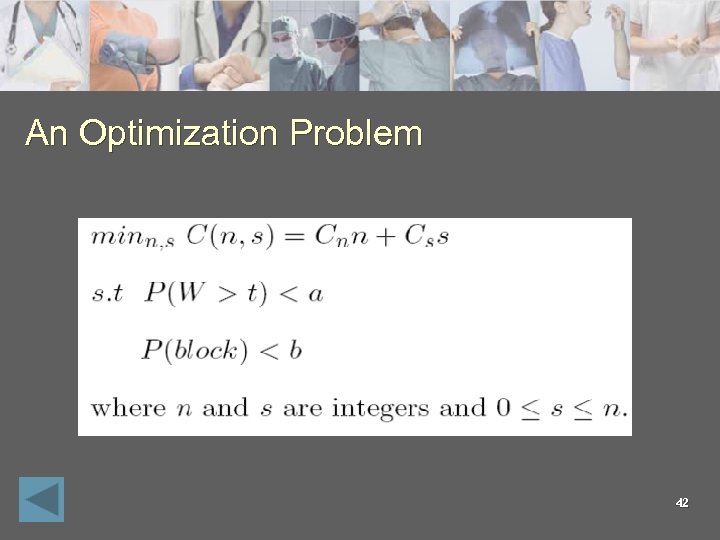
Research Objectives n n n Analyzing model for a Medical Unit with s nurses and n beds, which are partly/fully occupied by patients: semi-open queueing network with multiple statistically identical customers and servers. Questions addressed: How many servers (nurses) are required (staffing), and how many fixed resources (beds) are needed (allocation) in order to minimize costs while sustaining a certain service level? Coping with time-variability 4

We Follow n Basic: l l l n Analytical models in HC: l l n Halfin and Whitt (1981) Mandelbaum, Massey and Reiman (1998) Khudyakov (2006) Nurse staffing: Jennings and Véricourt (2007), Yankovic and Green (2007) Beds capacity: Green (2002, 2004) Service Engineering (mainly call centers): l Gans, Koole, Mandelbaum: “Telephone call centers: Tutorial, Review and Research prospects” 5

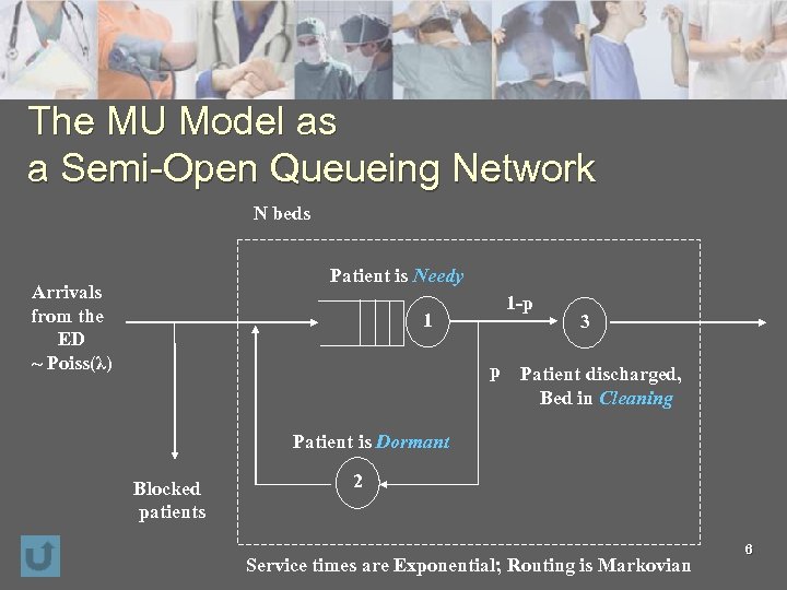The MU Model as a Semi-Open Queueing Network N beds Patient is Needy Arrivals from the ED ~ Poiss(λ) 1 1 -p 3 p Patient discharged, Bed in Cleaning Patient is Dormant Blocked patients 2 Service times are Exponential; Routing is Markovian 6

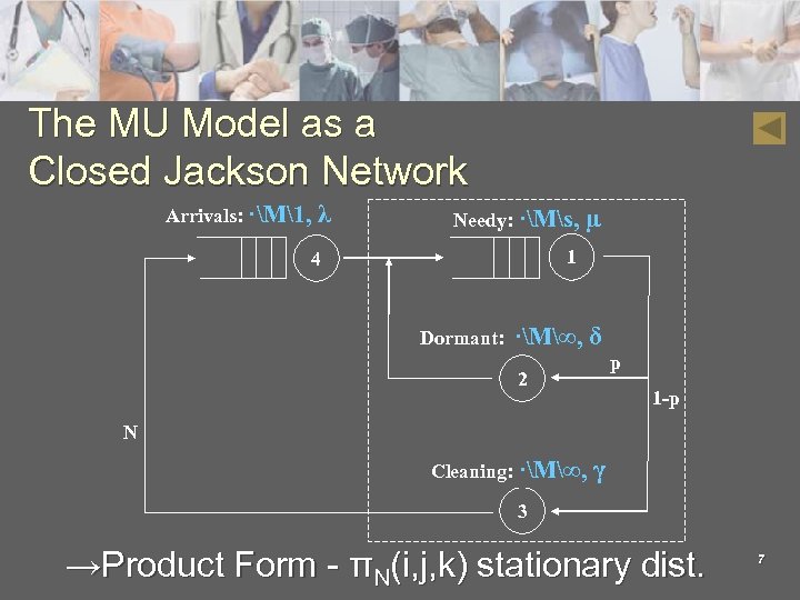The MU Model as a Closed Jackson Network Arrivals: ·M1, λ Needy: ·Ms, µ 1 4 Dormant: ·M∞, δ p 2 1 -p N Cleaning: ·M∞, γ 3 →Product Form - πN(i, j, k) stationary dist. 7

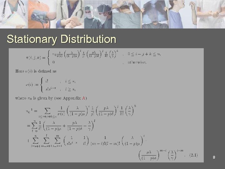Stationary Distribution 8

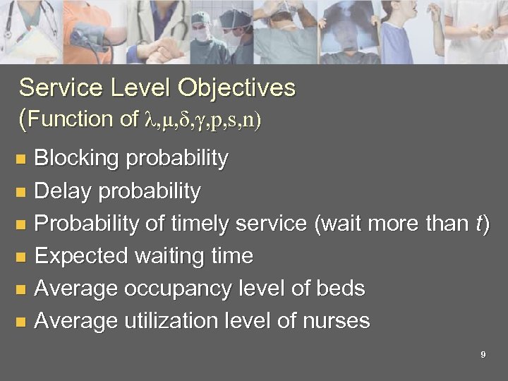Service Level Objectives (Function of λ, μ, δ, γ, p, s, n) Blocking probability n Delay probability n Probability of timely service (wait more than t) n Expected waiting time n Average occupancy level of beds n Average utilization level of nurses n 9

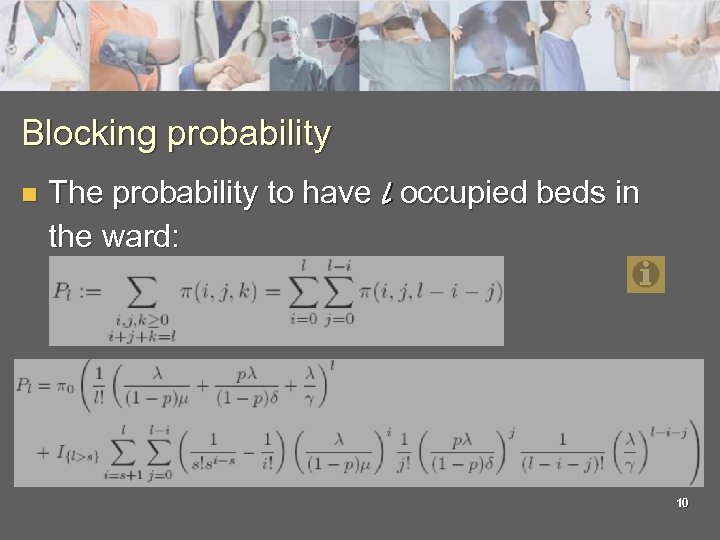Blocking probability n The probability to have l occupied beds in the ward: 10

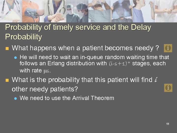Probability of timely service and the Delay Probability n What happens when a patient becomes needy ? l n He will need to wait an in-queue random waiting time that follows an Erlang distribution with (i-s+1)+ stages, each with rate μs. What is the probability that this patient will find i other needy patients? l We need to use the Arrival Theorem 11

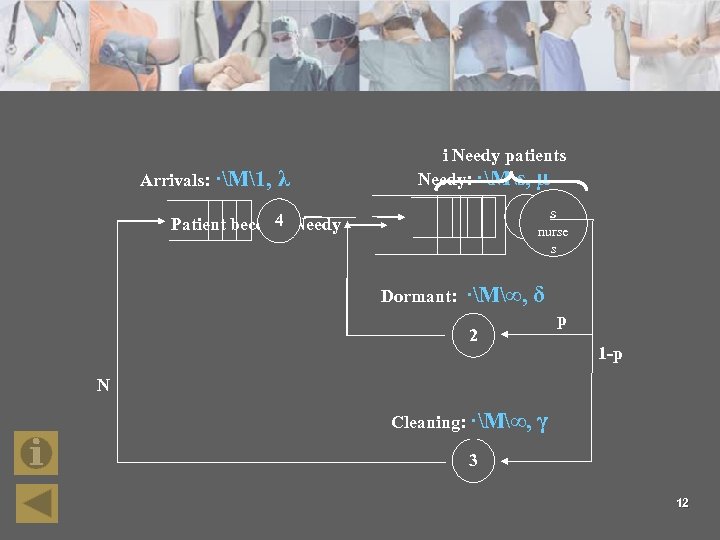Arrivals: ·M1, λ i Needy patients Needy: ·Ms, µ 1 4 Patient become Needy Dormant: s nurse s ·M∞, δ p 2 1 -p N Cleaning: ·M∞, γ 3 12

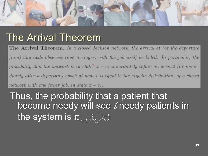The Arrival Theorem Thus, the probability that a patient that become needy will see i needy patients in the system is πn-1(i, j, k) 13

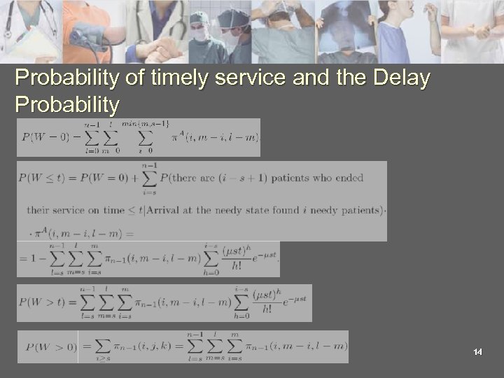Probability of timely service and the Delay Probability 14

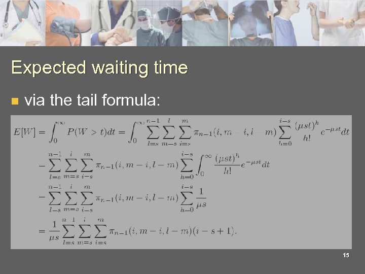Expected waiting time n via the tail formula: 15

QED Q’s: Quality- and Efficiency-Driven Queues n n n Traditional queueing theory predicts that servicequality and server’s efficiency must trade off against each other. Yet, one can balance both requirements carefully (Example: in well-run call-centers, 50% served “immediately”, along with over 90% agent’s utilization, is not uncommon) This is achieved in a special asymptotic operational regime – the QED regime 16

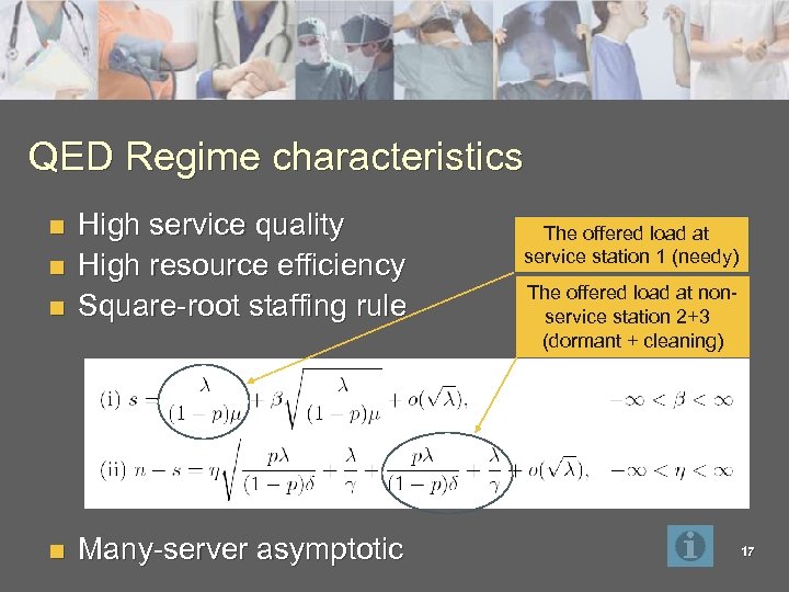QED Regime characteristics n High service quality High resource efficiency Square-root staffing rule n Many-server asymptotic n n The offered load at service station 1 (needy) The offered load at nonservice station 2+3 (dormant + cleaning) 17

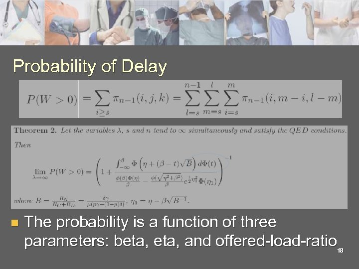Probability of Delay n The probability is a function of three parameters: beta, and offered-load-ratio 18

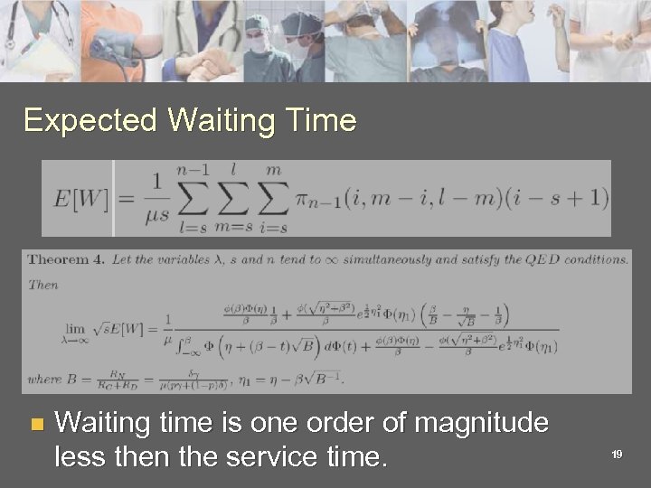Expected Waiting Time n Waiting time is one order of magnitude less then the service time. 19

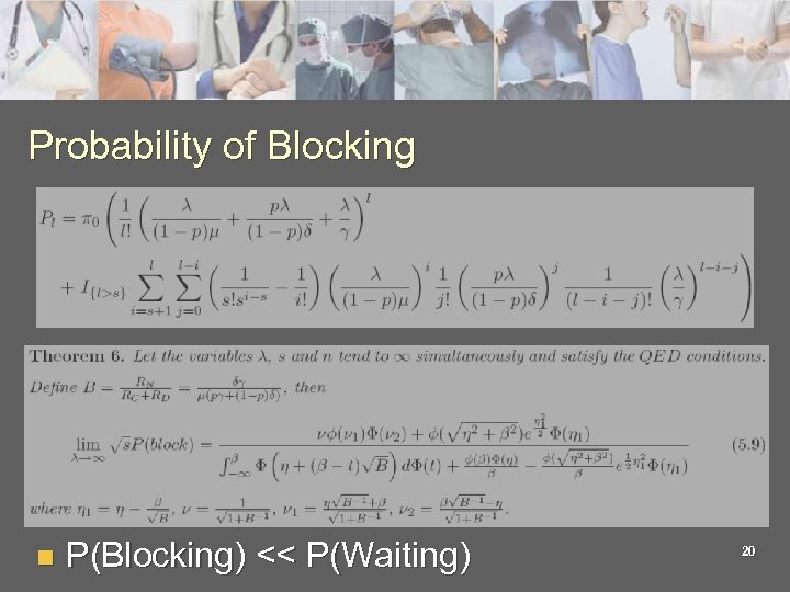Probability of Blocking n P(Blocking) << P(Waiting) 20

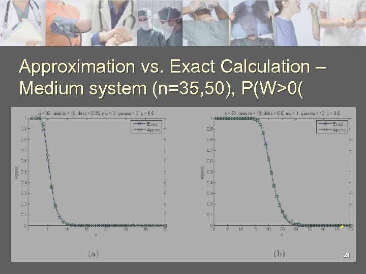Approximation vs. Exact Calculation – Medium system (n=35, 50), P(W>0( 21

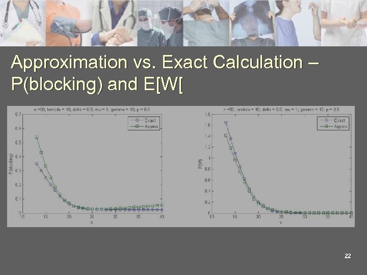Approximation vs. Exact Calculation – P(blocking) and E[W[ 22

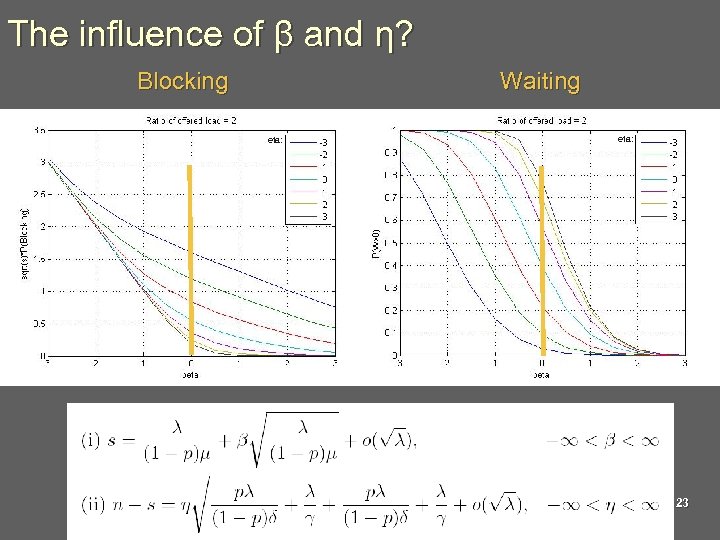The influence of β and η? Blocking Waiting eta: 23

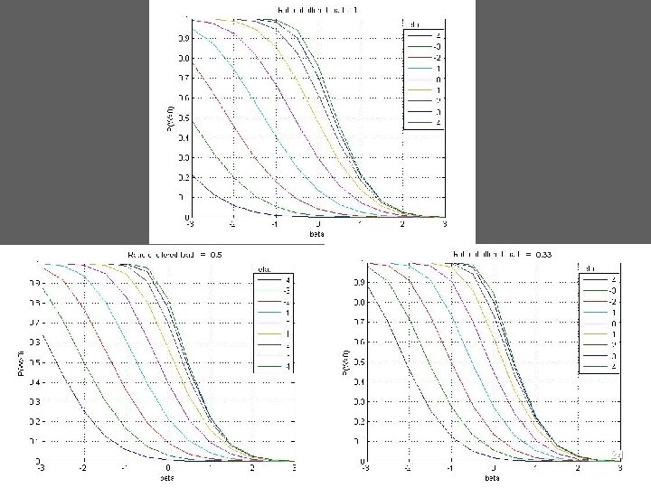= 0. 5 = 0. 33 24

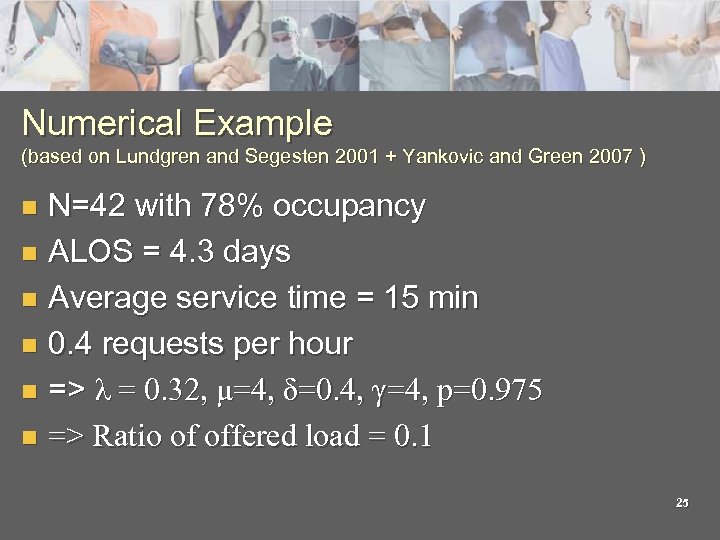Numerical Example (based on Lundgren and Segesten 2001 + Yankovic and Green 2007 ) N=42 with 78% occupancy n ALOS = 4. 3 days n Average service time = 15 min n 0. 4 requests per hour n => λ = 0. 32, μ=4, δ=0. 4, γ=4, p=0. 975 n => Ratio of offered load = 0. 1 n 25

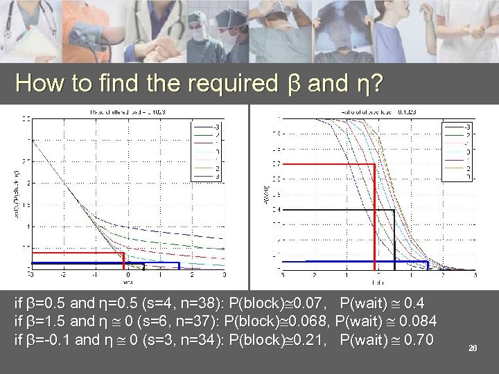How to find the required β and η? if β=0. 5 and η=0. 5 (s=4, n=38): P(block) 0. 07, P(wait) 0. 4 if β=1. 5 and η 0 (s=6, n=37): P(block) 0. 068, P(wait) 0. 084 if β=-0. 1 and η 0 (s=3, n=34): P(block) 0. 21, P(wait) 0. 70 26

Regime N S P(wait) P(blocking) E [W ] Nurses – QED; Beds-ED 7 4 0. 32 0. 84 0. 11 Nurses – QD ; Beds-ED 7 7 0 0. 83 0 Nurses – QED; Beds-QED 20 10 0. 44 0. 55 0. 11 Nurses – QD ; Beds-QED 20 15 0 0. 53 0 Nurses – ED ; Beds-ED 30 3 1 0. 85 7. 89 Nurses – QED; Beds-QED 30 14 0. 55 0. 35 0. 13 Nurses – QD ; Beds-QED 30 21 0 0. 31 0 Nurses – ED ; Beds-ED 50 3 1 0. 85 14. 56 Nurses – ED ; Beds-QED 50 10 1 0. 5 2. 85 Nurses – QED; Beds-QD 50 21 0. 5 0. 05 0. 12 Nurses – QD ; Beds-QD 50 31 0 0. 02 0 Lambda-10; Delta-0. 5; Mu-1; Gamma-10; p-0. 5; Ratio=1. 05 27

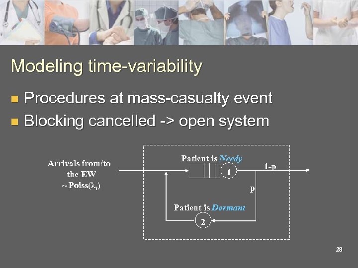Modeling time-variability Procedures at mass-casualty event n Blocking cancelled -> open system n Arrivals from/to the EW ~ Poiss(λt) Patient is Needy 1 -p 1 p Patient is Dormant 2 28

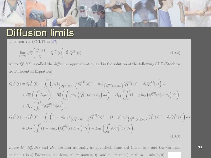
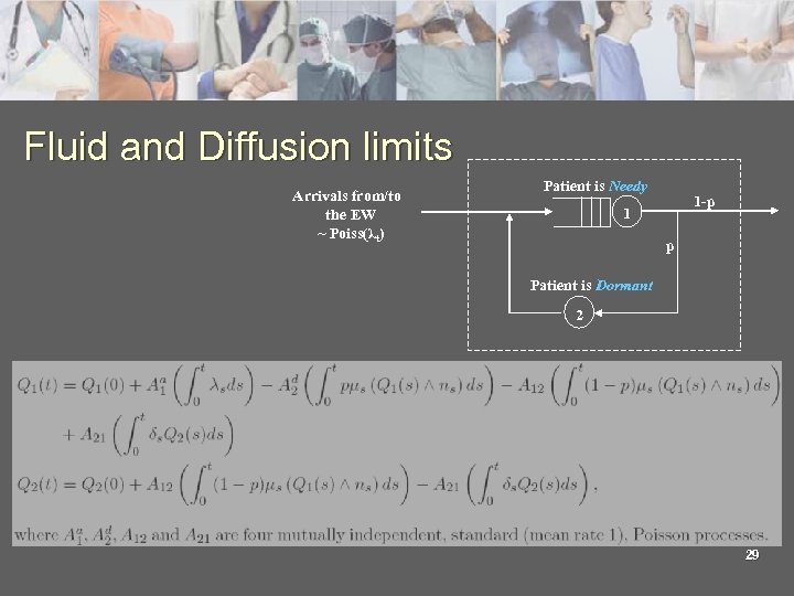Fluid and Diffusion limits Arrivals from/to the EW ~ Poiss(λt) Patient is Needy 1 -p 1 p Patient is Dormant 2 29

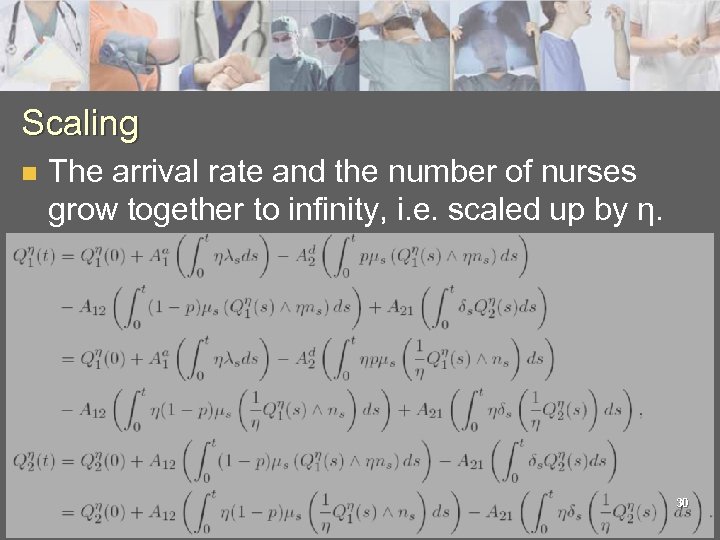Scaling n The arrival rate and the number of nurses grow together to infinity, i. e. scaled up by η. 30

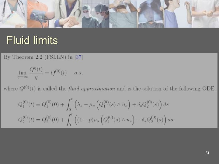Fluid limits 31

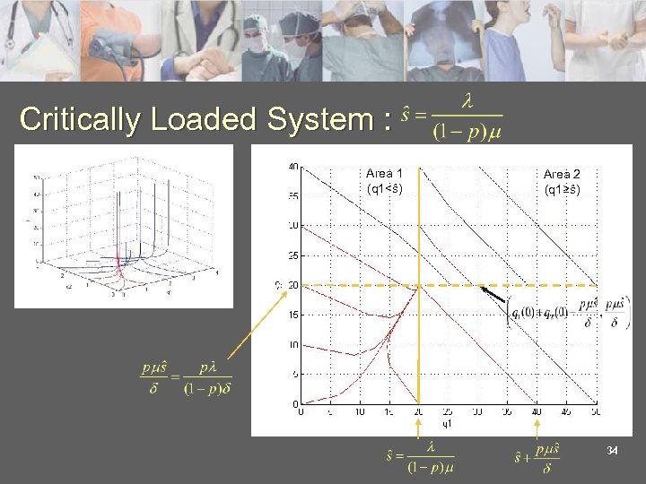
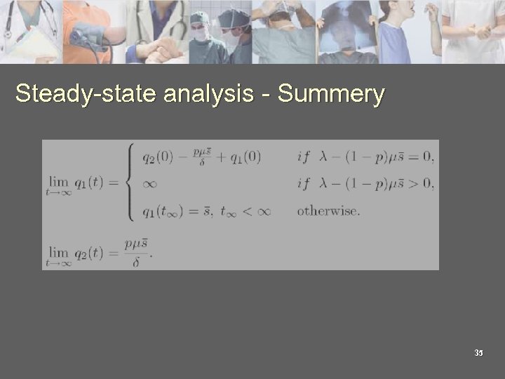
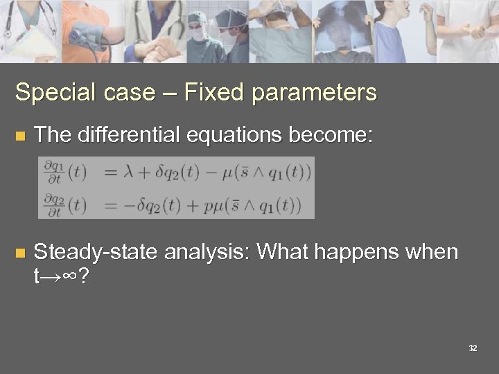Special case – Fixed parameters n The differential equations become: n Steady-state analysis: What happens when t→∞? 32

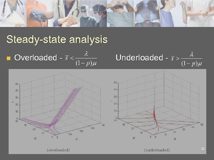Steady-state analysis n Overloaded - Underloaded - 33

Critically Loaded System : Area 1 (q 1<ŝ) Area 2 (q 1≥ŝ) 34

Steady-state analysis - Summery 35

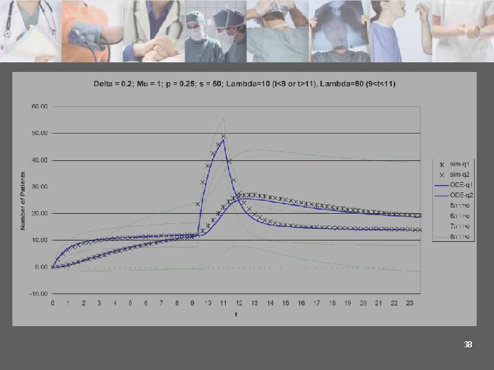
Diffusion limits 36

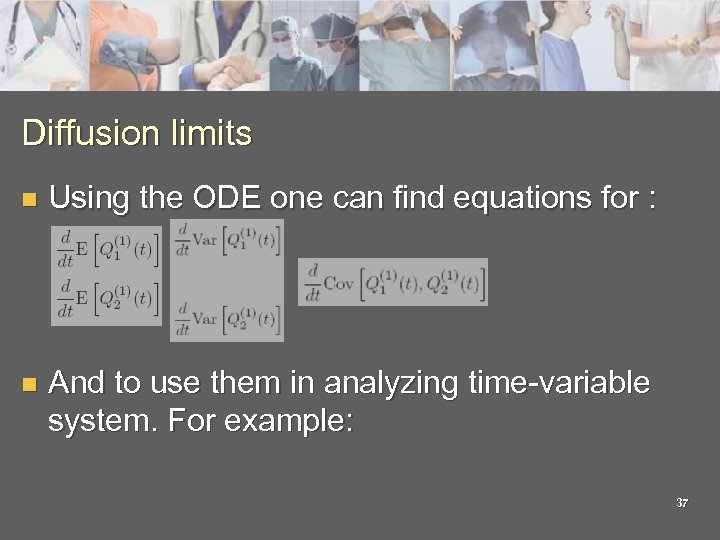Diffusion limits n Using the ODE one can find equations for : n And to use them in analyzing time-variable system. For example: 37

38

Future Research n Investigating approximation of closed system l n Optimization l l n n From which n are the approximations accurate? (simulation vs. rates of convergence) Solving the bed-nurse optimization problem Difference between hierarchical and simultaneous planning methods Validation of model using RFID data Expanding the model (Heterogeneous patients; adding doctors) 39

Thank you

Mandating minimum nurse-to-patient ratios Advantage: Ensures patient safety, reduces patients deaths, recruitment of new nurses, and stopping attrition. Disadvantage: Ratios are not flexible enough to allow hospitals to operate safely and efficiently The Wall Street Journal - Dec 2006 41

An Optimization Problem 42