Class 7.ppt
- Количество слайдов: 30
QUANTITATIVE METHODS OF BUSINESS RESEARCH Class 7. Topic 13. Instrumental variables regression.
Learning objectives and outcomes Understand the concept of endogeneity and the IV method as a way of obtaining consistent estimates. l Understand the necessary properties of a valid instrument. l Understand the properties of the IV estimator. l
Planned 13. 1. The IV estimator with a single regressor and a single instrument. 13. 2. The general IV regression model. 12. 3. Checking instrument validity.
Positioning of the method If the random errors are influenced by the Xvariables, then a possible approach is to identify Z-variables, that are highly correlated with X-variables, but not with the errors. These Z-variables are called Instrumental variables.
Instrumental Variables Regression IV can thus be used to address the following important threats to internal validity: l l Omitted variable bias from a variable that is correlated with X but is unobserved, so cannot be included in the regression; Simultaneous causality bias (endogenous explanatory variables; X causes Y, Y causes X); Errors-in-variables bias (X is measured with error) Instrumental variables regression can eliminate bias from these three sources
Terminology: Endogeneity and Exogeneity An endogenous variable is one that is correlated with ε An exogenous variable is one that is uncorrelated with ε. Historical note: “Endogenous” literally means “determined within the system, ” that is, a variable that is jointly determined with Y, that is, a variable subject to simultaneous causality. However, this definition is narrow and IV regression can be used to address OV bias and errors-in-variable bias, not just to simultaneous causality bias.
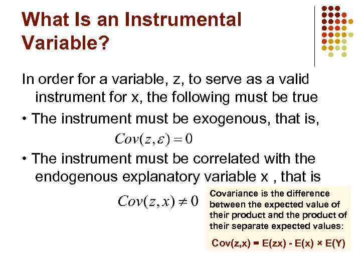
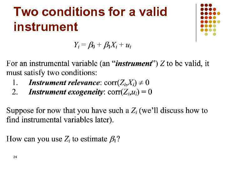
What Is an Instrumental Variable? In order for a variable, z, to serve as a valid instrument for x, the following must be true • The instrument must be exogenous, that is, • The instrument must be correlated with the endogenous explanatory variable x , that is Covariance is the difference between the expected value of their product and the product of their separate expected values: Cov(z, x) = E(zx) - E(x) × E(Y)
Two-Stage Least Squares (TSLS) Two step process: 1) regress the endogenous regressor(s) on all the exogenous variables; 2) use the predicted values from step 1 as replacement for the endogenous regressor in the original equation. This instrumental variable procedure is referred to as Two-Stage Least Squares (TSLS)
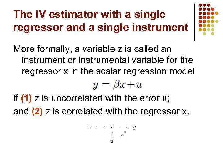
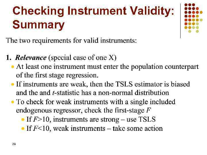
The IV estimator with a single regressor and a single instrument More formally, a variable z is called an instrument or instrumental variable for the regressor x in the scalar regression model if (1) z is uncorrelated with the error u; and (2) z is correlated with the regressor x.
Examples of an Instrument Suppose we want to estimate the response of market demand to exogenous changes in market price. Quantity demanded clearly depends on price, but prices are not exogenously given since they are determined in part by market demand. A suitable instrument for price is a variable that is correlated with price but does not directly effect quantity demanded. An obvious candidate is a variable that effects market supply, since this also effect prices, but is not a direct determinant of demand.
Examples of an Instrument For the public health example, we might use per capita income in each city as an instrument or z variable. It is likely to influence public health expenditure, as cities with a larger tax base might be expected to spend more on all services, and will not be directly affected by the unobserved factors in the primary relationship.
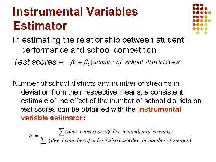
Instrumental Variables Estimator In estimating the relationship between student performance and school competition Test scores = Number of school districts and number of streams in deviation from their respective means, a consistent estimate of the effect of the number of school districts on test scores can be obtained with the instrumental variable estimator:
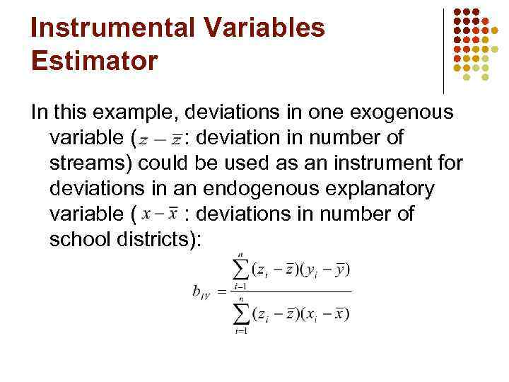
Instrumental Variables Estimator In this example, deviations in one exogenous variable ( : deviation in number of streams) could be used as an instrument for deviations in an endogenous explanatory variable ( : deviations in number of school districts):
Planned 13. 1. The IV estimator with a single regressor and a single instrument. 13. 2. The general IV regression model. 12. 3. Checking instrument validity.
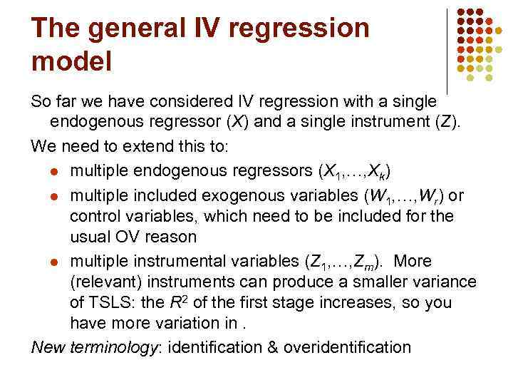
The general IV regression model So far we have considered IV regression with a single endogenous regressor (X) and a single instrument (Z). We need to extend this to: l multiple endogenous regressors (X 1, …, Xk) l multiple included exogenous variables (W 1, …, Wr) or control variables, which need to be included for the usual OV reason l multiple instrumental variables (Z 1, …, Zm). More (relevant) instruments can produce a smaller variance of TSLS: the R 2 of the first stage increases, so you have more variation in. New terminology: identification & overidentification
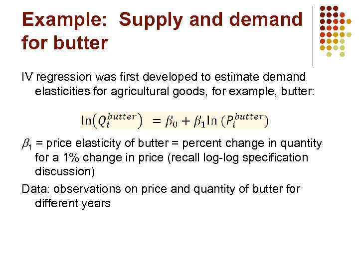
Example: Supply and demand for butter IV regression was first developed to estimate demand elasticities for agricultural goods, for example, butter: 1 = price elasticity of butter = percent change in quantity for a 1% change in price (recall log-log specification discussion) Data: observations on price and quantity of butter for different years
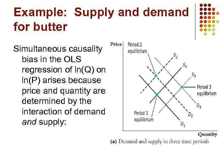
Example: Supply and demand for butter Simultaneous causality bias in the OLS regression of ln(Q) on ln(P) arises because price and quantity are determined by the interaction of demand supply:

Example: Supply and demand for butter Let Z = rainfall in dairy-producing regions. Is Z a valid instrument? (1) Relevant? corr(raini, ln(P)) ≠ 0? insufficient rainfall means less grazing means less butter means higher prices (2) Exogenous? corr(raini, ui) = 0? whether it rains in dairy-producing regions shouldn’t affect demand for butter
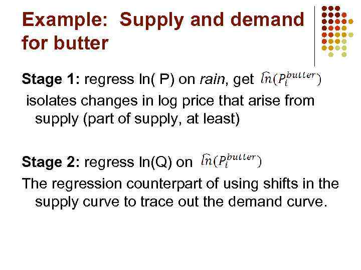
Example: Supply and demand for butter Stage 1: regress ln( P) on rain, get isolates changes in log price that arise from supply (part of supply, at least) Stage 2: regress ln(Q) on The regression counterpart of using shifts in the supply curve to trace out the demand curve.
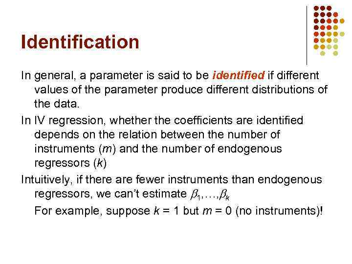
Identification In general, a parameter is said to be identified if different values of the parameter produce different distributions of the data. In IV regression, whether the coefficients are identified depends on the relation between the number of instruments (m) and the number of endogenous regressors (k) Intuitively, if there are fewer instruments than endogenous regressors, we can’t estimate 1, …, k For example, suppose k = 1 but m = 0 (no instruments)!
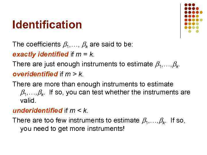
Identification The coefficients 1, …, k are said to be: exactly identified if m = k. There are just enough instruments to estimate 1, …, k. overidentified if m > k. There are more than enough instruments to estimate 1, …, k. If so, you can test whether the instruments are valid. underidentified if m < k. There are too few instruments to estimate 1, …, k. If so, you need to get more instruments!
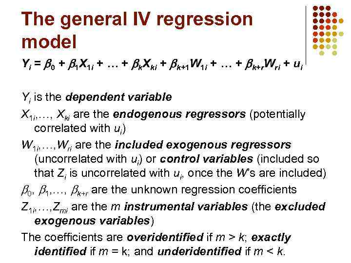
The general IV regression model Yi = 0 + 1 X 1 i + … + k. Xki + k+1 W 1 i + … + k+r. Wri + ui Yi is the dependent variable X 1 i, …, Xki are the endogenous regressors (potentially correlated with ui) W 1 i, …, Wri are the included exogenous regressors (uncorrelated with ui) or control variables (included so that Zi is uncorrelated with ui, once the W’s are included) 0, 1, …, k+r are the unknown regression coefficients Z 1 i, …, Zmi are the m instrumental variables (the excluded exogenous variables) The coefficients are overidentified if m > k; exactly identified if m = k; and underidentified if m < k.
Planned 13. 1. The IV estimator with a single regressor and a single instrument. 13. 2. The general IV regression model. 12. 3. Checking instrument validity.
Two conditions for a valid instrument 24
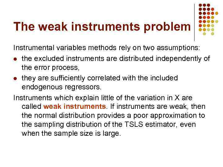
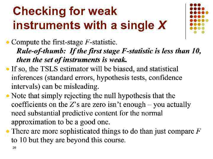
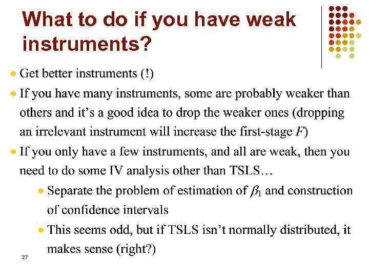
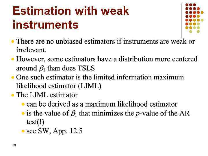
The weak instruments problem Instrumental variables methods rely on two assumptions: l the excluded instruments are distributed independently of the error process, l they are sufficiently correlated with the included endogenous regressors. Instruments which explain little of the variation in X are called weak instruments. If instruments are weak, then the normal distribution provides a poor approximation to the sampling distribution of the TSLS estimator, even when the sample size is large.
Checking for weak instruments with a single X 26
What to do if you have weak instruments? 27
Estimation with weak instruments 28
Checking Instrument Validity: Summary 29

Homework Reading: SW Ch. 12. 1 -12. 3. . Class and home exercises: Home assignment: 1. SW E 15. 2 (p. 668 -669) US_Macro_Monthly
Class 7.ppt