

317f9338536ed2f71ada6b59ddf986ae.ppt
- Количество слайдов: 81
 Quantitative genetics • • Many traits that are important in agriculture, biology and biomedicine are continuous in their phenotypes. For example, Crop Yield Stemwood Volume Plant Disease Resistances Body Weight in Animals Fat Content of Meat Time to First Flower IQ Blood Pressure
 The following image demonstrates the variation for flower diameter, number of flower parts and the color of the flower in Gaillaridia pilchella (Mc. Clean 1997). Each trait is controlled by a number of genes each interacting with each other and an array of environmental factors.
 Number of Genes Number of Genotypes 1 2 5 10 3 9 243 59, 049
 Consider two genes, A with two alleles A and a, and B with two alleles B and b. - Each of the alleles will be assigned metric values - We give the A allele 4 units and the a allele 2 units - At the other locus, the B allele will be given 2 units and the b allele 1 unit Genotype AABB AABb AAbb Aa. BB 2 Aa. Bb Aabb aa. BB aa. Bb aabb Ratio 1 2 1 4 2 1 Metric value 12 11 10 10 9 8 8 7 6
 A grapical format is used to present the above results:
 Normal distribution of a quantitative trait may be due to • Many genes • Environmental effects The traditional view: polygenes each with small effect and being sensitive to environments The new view: A few major gene and many polygenes (oligogenic control), interacting with environments
 Traditional quantitative genetics research: Variance component partitioning • The phenotypic variance of a quantitative trait can be partitioned into genetic and environmental variance components. • To understand the inheritance of the trait, we need to estimate the relative contribution of these two components. • We define the proportion of the genetic variance to the total phenotypic variance as the heritability (H 2). - If H 2 = 1. 0, then the trait is 100% controlled by genetics - If H 2 = 0, then the trait is purely affected by environmental factors.
 proposed a theory for partitioning genetic variance into additive, dominant") • Fisher (1918) proposed a theory for partitioning genetic variance into additive, dominant and epistatic components; • Cockerham (1954) explained these genetic variance components in terms of experimental variances (from ANOVA), which makes it possible to estimate additive and dominant components (but not the epistatic component); • I proposed a clonal design to estimate additive, dominant and part-of-epistatic variance components Wu, R. , 1996 Detecting epistatic genetic variance with a clonally replicated design: Models for low- vs. high-order nonallelic interaction. Theoretical and Applied Genetics 93: 102 -109.
• Fisher (1918) proposed a theory for partitioning genetic variance into additive, dominant and epistatic components; • Cockerham (1954) explained these genetic variance components in terms of experimental variances (from ANOVA), which makes it possible to estimate additive and dominant components (but not the epistatic component); • I proposed a clonal design to estimate additive, dominant and part-of-epistatic variance components Wu, R. , 1996 Detecting epistatic genetic variance with a clonally replicated design: Models for low- vs. high-order nonallelic interaction. Theoretical and Applied Genetics 93: 102 -109.
variances One-gene model Genotype Genotypic value Net genotypic value aa") Genetic Parameters: Means and (Co)variances One-gene model Genotype Genotypic value Net genotypic value aa Aa G 0 G 1 -a 0 d AA G 2 a origin=(G 0+G 2)/2 a = additive genotypic value d = dominant genotypic value Environmental deviation E 0 E 1 E 2 Phenotype or Phenotypic value Y 0=G 0+E 0 Y 1=G 1+E 1 Y 2=G 2+E 2 P 0 =q 2 -a - =-2 p[a+(q-p)d] P 1 P 2 =2 pq =p 2 d - a - =(q-p)[a+(q-p)d] Genotype frequency at HWE Deviation from population mean =2 q[a+(q-p)d] Letting =a+(q-p)d Breeding value Dominant deviation -2 p 2 d =-2 p -2 p 2 d +2 pqd -2 q 2 d =(q-p) +2 pqd =2 q -2 q 2 d (q-p) 2 pqd 2 q -2 q 2 d
Genetic Parameters: Means and (Co)variances One-gene model Genotype Genotypic value Net genotypic value aa Aa G 0 G 1 -a 0 d AA G 2 a origin=(G 0+G 2)/2 a = additive genotypic value d = dominant genotypic value Environmental deviation E 0 E 1 E 2 Phenotype or Phenotypic value Y 0=G 0+E 0 Y 1=G 1+E 1 Y 2=G 2+E 2 P 0 =q 2 -a - =-2 p[a+(q-p)d] P 1 P 2 =2 pq =p 2 d - a - =(q-p)[a+(q-p)d] Genotype frequency at HWE Deviation from population mean =2 q[a+(q-p)d] Letting =a+(q-p)d Breeding value Dominant deviation -2 p 2 d =-2 p -2 p 2 d +2 pqd -2 q 2 d =(q-p) +2 pqd =2 q -2 q 2 d (q-p) 2 pqd 2 q -2 q 2 d
 + 2 pqd + p 2 a = (p-q)a+2") Population mean = q 2(-a) + 2 pqd + p 2 a = (p-q)a+2 pqd Genetic variance 2 g = q 2(-2 p 2 d)2 + 2 pq[(q-p) +2 pqd]2 + p 2(2 q -2 q 2 d)2 = 2 pq 2 + (2 pqd)2 = 2 a (or VA) + 2 d (or VD) Additive genetic variance, Dominant genetic variance, depending on both on a and d depending only on d Phenotypic variance 2 P = q 2 Y 02 + 2 pq. Y 12 + p 2 Y 22 – (q 2 Y 0 + 2 pq. Y 1 + p 2 Y 2)2 Define H 2 = 2 g / 2 P as the broad-sense heritability h 2 = 2 a / 2 P as the narrow-sense heritability These two heritabilities are important in understanding the relative contribution of genetic and environmental factors to the overall phenotypic variance.
Population mean = q 2(-a) + 2 pqd + p 2 a = (p-q)a+2 pqd Genetic variance 2 g = q 2(-2 p 2 d)2 + 2 pq[(q-p) +2 pqd]2 + p 2(2 q -2 q 2 d)2 = 2 pq 2 + (2 pqd)2 = 2 a (or VA) + 2 d (or VD) Additive genetic variance, Dominant genetic variance, depending on both on a and d depending only on d Phenotypic variance 2 P = q 2 Y 02 + 2 pq. Y 12 + p 2 Y 22 – (q 2 Y 0 + 2 pq. Y 1 + p 2 Y 2)2 Define H 2 = 2 g / 2 P as the broad-sense heritability h 2 = 2 a / 2 P as the narrow-sense heritability These two heritabilities are important in understanding the relative contribution of genetic and environmental factors to the overall phenotypic variance.
d? It is the average effect due to the substitution of") What is = a+(q-p)d? It is the average effect due to the substitution of gene from one allele (A say) to the other (a). Event A a contains two possibilities From Aa to aa Frequency q Value change d-(-a) = q[d-(-a)]+p(a-d) = a+(q-p)d From AA to Aa p a-d
What is = a+(q-p)d? It is the average effect due to the substitution of gene from one allele (A say) to the other (a). Event A a contains two possibilities From Aa to aa Frequency q Value change d-(-a) = q[d-(-a)]+p(a-d) = a+(q-p)d From AA to Aa p a-d
 Midparent-offspring correlation __________________________________ Progeny Genotype Freq. of Midparent AA Aa aa Mean value of parents matings value a d -a of progeny __________________________________ AA × AA p 4 a 1 a AA × Aa 4 p 3 q ½(a+d) ½ ½ ½(a+d) AA × aa 2 p 2 q 2 0 1 d Aa × Aa 4 p 2 q 2 d ¼ ½d Aa × aa 4 pq 3 ½(-a+d) ½ ½ ½(-a+d) aa × aa q 4 -a 1 -a ________________________
 = E(OP) – E(O)E(P) = p") Covariance between midparent and offspring: _ _ Cov(OP) = E(OP) – E(O)E(P) = p 4 a a + 4 p 3 q ½(a+d) + … + q 4 (-a) – [(p-q)a+2 pqd]2 = pq 2 = ½ 2 a The regression of offspring on midparent values is _ _ b = Cov(OP)/ 2(P) = ½ 2 a / ½ 2 P = 2 a / 2 P = h 2 where 2(P¯)=½ 2 P is the variance of midparent value.
Covariance between midparent and offspring: _ _ Cov(OP) = E(OP) – E(O)E(P) = p 4 a a + 4 p 3 q ½(a+d) + … + q 4 (-a) – [(p-q)a+2 pqd]2 = pq 2 = ½ 2 a The regression of offspring on midparent values is _ _ b = Cov(OP)/ 2(P) = ½ 2 a / ½ 2 P = 2 a / 2 P = h 2 where 2(P¯)=½ 2 P is the variance of midparent value.
 IMPORTANT The regression of offspring on midparent values can be used to measure the heritability! This is a fundamental contribution by R. A. Fisher.
 You can derive other relationships Degree of relationship Covariance __________________________ Offspring and one parent Cov(OP) = 2 a/2 Half siblings Cov(FS) = 2 a/4 Full siblings Cov(FS) = 2 a/2 + 2 d/4 Monozygotic twins Cov(MT) = 2 a + 2 d Nephew and uncle Cov(NU) = 2 a/4 First cousins Cov(FC) = 2 a /8 Double first cousins Cov(DFC) = 2 a/4 + 2 d/16 Offspring and midparent Cov(O) = 2 a/2 __________________________
: A chromosomal segments that contribute to variation") QTL Mapping • Quantitative Trait Loci (QTL): A chromosomal segments that contribute to variation in a quantitative phenotype Lander, E. S. & Botstein, D. (1989). Mapping Mendelian factors underlying quantitative traits using RFLP linkage maps. Genetics 121, 185 -199.
QTL Mapping • Quantitative Trait Loci (QTL): A chromosomal segments that contribute to variation in a quantitative phenotype Lander, E. S. & Botstein, D. (1989). Mapping Mendelian factors underlying quantitative traits using RFLP linkage maps. Genetics 121, 185 -199.
 Maize Teosinte tb-1/tb-1 mutant maize
 in the F 2 hybrids between maize and teosinte") Mapping Quantitative Trait Loci (QTL) in the F 2 hybrids between maize and teosinte
Mapping Quantitative Trait Loci (QTL) in the F 2 hybrids between maize and teosinte
 The role of barren stalk 1") Nature 432, 630 - 635 (02 December 2004) The role of barren stalk 1 in the architecture of maize ANDREA GALLAVOTTI(1, 2), QIONG ZHAO(3), JUNKO KYOZUKA(4), ROBERT B. MEELEY(5), MATTHEW K. RITTER 1, *, JOHN F. DOEBLEY(3), M. ENRICO PÈ(2) & ROBERT J. SCHMIDT(1) 1 Section of Cell and Developmental Biology, University of California, San Diego, La Jolla, California 92093 -0116, USA 2 Dipartimento di Scienze Biomolecolari e Biotecnologie, Università degli Studi di Milano, 20133 Milan, Italy 3 Laboratory of Genetics, University of Wisconsin, Madison, Wisconsin 53706, USA 4 Graduate School of Agriculture and Life Science, The University of Tokyo, Tokyo 113 -8657, Japan 5 Crop Genetics Research, Pioneer-A Du. Pont Company, Johnston, Iowa 50131, USA * Present address: Biological Sciences Department, California Polytechnic State University, San Luis Obispo, California 93407, USA
Nature 432, 630 - 635 (02 December 2004) The role of barren stalk 1 in the architecture of maize ANDREA GALLAVOTTI(1, 2), QIONG ZHAO(3), JUNKO KYOZUKA(4), ROBERT B. MEELEY(5), MATTHEW K. RITTER 1, *, JOHN F. DOEBLEY(3), M. ENRICO PÈ(2) & ROBERT J. SCHMIDT(1) 1 Section of Cell and Developmental Biology, University of California, San Diego, La Jolla, California 92093 -0116, USA 2 Dipartimento di Scienze Biomolecolari e Biotecnologie, Università degli Studi di Milano, 20133 Milan, Italy 3 Laboratory of Genetics, University of Wisconsin, Madison, Wisconsin 53706, USA 4 Graduate School of Agriculture and Life Science, The University of Tokyo, Tokyo 113 -8657, Japan 5 Crop Genetics Research, Pioneer-A Du. Pont Company, Johnston, Iowa 50131, USA * Present address: Biological Sciences Department, California Polytechnic State University, San Luis Obispo, California 93407, USA
 Effects of ba 1 mutations on maize development Mutant Wild type No tassel Tassel
 A putative QTL affecting height in BC Sam- ple 1 2 3 4 5 6 7 8 Height (cm, y) 184 185 180 182 167 169 165 166 QTL genotype Qq (1) qq (0) If the QTL genotypes are known for each sample, as indicated at the left, then a simple ANOVA can be used to test statistical significance.
 x qq (P 2)") Suppose a backcross design Parent F 1 QQ (P 1) x qq (P 2) Qq x qq (P 2) BC Genetic effect Genotypic value Qq qq a* +a* 0
Suppose a backcross design Parent F 1 QQ (P 1) x qq (P 2) Qq x qq (P 2) BC Genetic effect Genotypic value Qq qq a* +a* 0
 QTL regression model The phenotypic value for individual i affected by a QTL can be expressed as, yi = + a* x*i + ei where is the overall mean, x*i is the indicator variable for QTL genotypes, defined as x*i = 1 for Qq x*i is missing 0 for qq, a* is the “real” effect of the QTL and ei is the residual error, ei ~ N(0, 2).
 1 184 2 185") Data format for a backcross Sam- Height ple (cm, y) 1 184 2 185 3 180 4 182 5 167 6 169 7 165 8 166 Complete data = Marker genotype QTL M 1 M 2 Mm (1) Nn (1) Mm (1) nn (0) ½ mm (0) Nn (1) Observed data + Qq ½ ½ ½ ½ qq ½ ½ Missing data
Data format for a backcross Sam- Height ple (cm, y) 1 184 2 185 3 180 4 182 5 167 6 169 7 165 8 166 Complete data = Marker genotype QTL M 1 M 2 Mm (1) Nn (1) Mm (1) nn (0) ½ mm (0) Nn (1) Observed data + Qq ½ ½ ½ ½ qq ½ ½ Missing data
 Two statistical models I - Marker regression model yi = + axi + ei where • xi is the indicator variable for marker genotypes defined as xi = 1 for Mm 0 for mm , • a is the “effect” of the marker (but the marker has no effect. There is the a because of the existence of a putative QTL linked with the marker) • ei ~ N(0, 2)
 Marker group Sample size Sample mean Sample") Heights classified by markers (say marker 1) Marker group Sample size Sample mean Sample variance Mm mm n 1 = 4 n 0 = 4 m 1=182. 75 s 21= 4. 92 m 0=166. 75 s 20= 2. 92
Heights classified by markers (say marker 1) Marker group Sample size Sample mean Sample variance Mm mm n 1 = 4 n 0 = 4 m 1=182. 75 s 21= 4. 92 m 0=166. 75 s 20= 2. 92
 The hypothesis for the association between the marker and QTL H 0: m 1 = m 0 H 1: m 1 m 0 Calculate the test statistic: t = (m 1–m 0)/ [s 2(1/n 1+1/n 0)] = (182. 75 -165. 75)/ [3. 92(1/4+1/4)] = 11. 43, where s 2 = [(n 1 -1)s 21+(n 0 -1)s 20]/(n 1+n 0– 2) = [(4 -1)4. 92 + (4 -1)2. 92]/(4+4 -2) = 3. 92 Compare t with the critical value tdf=n 1+n 2 -2(0. 05) = 1. 94 from the t-table. If t > tdf=n 1+n 2 -2 (0. 05), we reject H 0 at the significance level 0. 05 there is a QTL If t < tdf=n 1+n 2 -2 (0. 05), we accept H 0 at the significance level 0. 05 there is no QTL
 Why can the t-test probe a QTL? • • Assume a backcross with two genes, one marker (alleles M and m) and one QTL (allele Q and q). These two genes are linked with the recombination fraction of r. Frequency Mean effect Mm. Qq (1 -r)/2 m+a Mmqq r/2 m mm. Qq r/2 m+a mmqq (1 -r)/2 m Mean of marker genotype Mm: m 1= [(1 -r)/2 (m+a) + r/2 m]/(1/2) = m + (1 -r)a Mean of marker genotype mm: m 0= [r/2 (m+a) + (1 -r)/2 m]/(1/2) = m + ra The difference m 1 – m 0 = m + (1 -r)a – m – ra = (1 -2 r)a
 • The difference of marker genotypes can reflect the size of the QTL, • This reflection is confounded by the recombination fraction Based on the t-test, we cannot distinguish between the two cases, - Large QTL genetic effect but loose linkage with the marker - Small QTL effect but tight linkage with the marker
 Example: marker analysis for body weight in a backcross of mice ___________________________________ Marker class 1 Marker class 0 ___________ Marker n 1 m 1 s 2 1 n 0 m 0 s 2 0 t p-value _______________________________________ 1 Hmg 1 -rs 13 41 54. 20 111. 81 62 47. 32 63. 67 3. 754 <0. 01 2 DXMit 57 42 55. 21 104. 12 61 46. 51 56. 12 4. 99 <0. 01 3 Rps 17 -rs 11 43 55. 30 101. 98 60 46. 30 54. 38 5. 231 <0. 000001 ___________________________________
 Marker analysis for the F 2 In the F 2 there are three marker genotypes, MM, Mm and mm, which allow for the test of additive and dominant genetic effects. Genotype MM: Mm: mm: m 2 m 1 m 0 Mean s 22 s 21 s 20 Variance
 Testing for the additive effect H 0: m 2 = m 0 H 1: m 2 m 0 t 1 = (m 2–m 0)/ [s 2(1/n 2+1/n 0)], where s 2 = [(n 2 -1)s 22+(n 0 -1)s 20]/(n 1+n 0– 2) Compare it with tdf=n 2+n 0 -2(0. 05)
 Testing for the dominant effect H 0: m 1 = (m 2 + m 0)/2 H 1: m 1 (m 2 + m 0)/2 t 2 = [m 1–(m 2 + m 0)/2]/ {[s 2[1/n 1+1/(4 n 2)+1/(4 n 0)]], where s 2 = [(n 2 -1)s 22+(n 1 -1)s 21+(n 0 -1)s 20]/(n 2+n 1+n 0– 3) Compare it with tdf=n 2+n 1+n 0 -3(0. 05)
 Example: Marker analysis in an F 2 of maize _______________________________________________ Marker class 2 Marker class 1 Marker class 0 Additive Dominant ______ ______________ M n 2 m 2 s 22 n 1 m 1 s 21 n 0 m 0 s 20 t 1 p-value t 2 p-value ________________________________________________ 1 43 5. 24 2. 44 86 4. 27 2. 93 42 3. 11 2. 76 6. 10 <0. 001 0. 38 0. 70 2 48 4. 82 3. 15 89 4. 17 3. 26 34 3. 54 2. 84 3. 28 0. 001 -0. 05 0. 96 3 42 5. 01 3. 23 92 4. 14 3. 18 37 3. 57 2. 68 3. 71 0. 0002 -0. 57 ________________________________________________
 Suppose gene order Marker") II – QTL regression model based on markers (interval mapping) Suppose gene order Marker 1 – QTL – Marker 2 yi = + a*zi + ei where • a* is the “real” effect of a QTL, • zi is an indicator variable describing the probability of individual i to carry the QTL genotype, Qq or qq, given a possible marker genotype, • ei ~ N(0, 2)
II – QTL regression model based on markers (interval mapping) Suppose gene order Marker 1 – QTL – Marker 2 yi = + a*zi + ei where • a* is the “real” effect of a QTL, • zi is an indicator variable describing the probability of individual i to carry the QTL genotype, Qq or qq, given a possible marker genotype, • ei ~ N(0, 2)
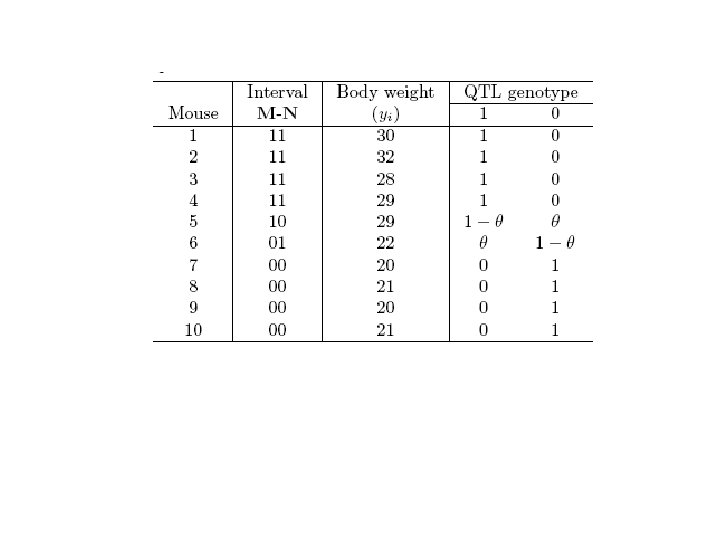
 1 2 genotype") Indicators for a backcross Sam- Height Markers Three-locus ple (cm, yi) 1 2 genotype 1 184 1 1 111 101 2 185 1 1 111 101 3 180 1 1 111 101 4 182 1 0 110 100 5 167 0 1 001 011 6 169 0 0 000 010 7 165 0 0 000 010 8 166 0 0 000 010 QTL x*i 1 Marker QTL|marker xi zi 1 1 P(1|11) 1 1 1 0 P(1|10) 1 - 0 0 1 0 0 0 P(1|01) P(1|00)
Indicators for a backcross Sam- Height Markers Three-locus ple (cm, yi) 1 2 genotype 1 184 1 1 111 101 2 185 1 1 111 101 3 180 1 1 111 101 4 182 1 0 110 100 5 167 0 1 001 011 6 169 0 0 000 010 7 165 0 0 000 010 8 166 0 0 000 010 QTL x*i 1 Marker QTL|marker xi zi 1 1 P(1|11) 1 1 1 0 P(1|10) 1 - 0 0 1 0 0 0 P(1|01) P(1|00)
 of the QTL genotypes (missing) based on marker") Conditional probabilities ( 1|i or 0|i) of the QTL genotypes (missing) based on marker genotypes (observed) Marker Genotype 11 10 01 00 QTL genotype Freq. Qq(1) qq(0) ½(1 -r) (1 -r 1)(1 -r 2)/(1 -r) r 1 r 2/(1 -r) 1 0 ½r (1 -r 1)r 2/r r 1(1 -r 2)/r 1 - = 1 -r 1/r = r 1/r ½r r 1(1 -r 2)/r (1 -r 1)r 2/r 1 - ½(1 -r) r 1 r 2/(1 -r) (1 -r 1)(1 -r 2)/(1 -r) 0 1 Order Marker 1–QTL–Marker 2 r is the recombination fraction between two markers r 1 is the recombination fraction between marker 1 and QTL r 2 is the recombination fraction between QTL and marker 2
Conditional probabilities ( 1|i or 0|i) of the QTL genotypes (missing) based on marker genotypes (observed) Marker Genotype 11 10 01 00 QTL genotype Freq. Qq(1) qq(0) ½(1 -r) (1 -r 1)(1 -r 2)/(1 -r) r 1 r 2/(1 -r) 1 0 ½r (1 -r 1)r 2/r r 1(1 -r 2)/r 1 - = 1 -r 1/r = r 1/r ½r r 1(1 -r 2)/r (1 -r 1)r 2/r 1 - ½(1 -r) r 1 r 2/(1 -r) (1 -r 1)(1 -r 2)/(1 -r) 0 1 Order Marker 1–QTL–Marker 2 r is the recombination fraction between two markers r 1 is the recombination fraction between marker 1 and QTL r 2 is the recombination fraction between QTL and marker 2
 Interval mapping with regression approach • Consider a marker interval M 1 -M 2. We assume that a QTL is located at a particular position between the two markers (r 1 and are fixed) • With response variable, yi, and dependent variable, zi, a regression model is constructed as yi = + a*zi + ei • Statistical software, like SAS, can be used to estimate the parameters ( , a*, 2) for a particular QTL position contained in the regression model Matrix expression y = Z T + e y = (y 1, …, yn)T, e = (e 1, …, en)T Z = (Z 1, …, Zn)T, Zi = (1, zi), = ( , a*) E(e) = 0, V(e) = 2 I, I is an (n x n) identity matrix Estimates: = (ZTZ)-1 ZTy 2 = (1/n)(y-Z T)T(y-Z T)
 Model with no QTL: yi^") QTL model: yi^ = ^ + a*^zi (full model) Model with no QTL: yi^ = ^ (reduced model) Total sum of squares (SST) is the sum of (yi - ^)2 Residual sum of squares (SSE) is the sum of (yi - ^ - a*^zi)2 A test statistic for this method is for an experiment with n observations is LR = n ln(SST/SSE) Or F-value F = [(SST-SSE)/(2 -1)]/[SSE/(n-2)], compare the F value with F(1, n-2)(0. 05) Move the QTL position every 2 c. M from M 1 to M 2 and draw the profile of the F value. The peak of the profile corresponds to the best estimate of the QTL position. F-value M 1 M 2 M 3 M 4 M 5 Testing position
QTL model: yi^ = ^ + a*^zi (full model) Model with no QTL: yi^ = ^ (reduced model) Total sum of squares (SST) is the sum of (yi - ^)2 Residual sum of squares (SSE) is the sum of (yi - ^ - a*^zi)2 A test statistic for this method is for an experiment with n observations is LR = n ln(SST/SSE) Or F-value F = [(SST-SSE)/(2 -1)]/[SSE/(n-2)], compare the F value with F(1, n-2)(0. 05) Move the QTL position every 2 c. M from M 1 to M 2 and draw the profile of the F value. The peak of the profile corresponds to the best estimate of the QTL position. F-value M 1 M 2 M 3 M 4 M 5 Testing position
 Interval mapping with maximum likelihood • • • Linear regression model for specifying the effect of a putative QTL on a quantitative trait Mixture model-based likelihood Conditional probabilities of the QTL genotypes (missing) based on marker genotypes (observed) Normal distributions of phenotypic values for each QTL genotype group Log-likelihood equations (via differentiation) EM algorithm Log-likelihood ratios The profile of log-likelihood ratios across a linkage group The determination of thresholds Result interpretations
 Linear regression model for specifying the effect of a QTL on a quantitative trait yi = + a*zi + ei, i = 1, …, n (latent model) • • • a* is the (additive) effect of the putative QTL on the trait, zi is the indicator variable and defined as 1 when QTL genotype is Qq and 0 when QTL genotype is qq, ei N(0, 2) Observed data: Missing data: Parameters: • yi and marker genotypes M QTL genotypes = ( , a*, 2, =r 1/r) Observed marker genotypes and missing QTL genotypes are connected in terms of the conditional probability ( 1|i or 0|i) of QTL genotypes (Qq or qq), conditional upon marker genotypes (11, 10, 01 or 00).
 = i=1 n [½f 1(yi) +") Mixture model-based likelihood without marker information L( |y) = i=1 n [½f 1(yi) + ½f 0(yi)] Sample 1 2 3 4 5 6 7 8 Height (cm, y) 184 185 180 182 167 169 165 166 QTL genotype Qq qq ½ ½ ½ ½ Likelihood L 1 = ½f 1(y 1) + ½f 0(y 1) L 2 = ½f 1(y 2) + ½f 0(y 2) L 3 = ½f 1(y 3) + ½f 0(y 3) L 4 = ½f 1(y 4) + ½f 0(y 4) L 5 = ½f 1(y 5) + ½f 0(y 5) L 6 = ½f 1(y 6) + ½f 0(y 6) L 7 = ½f 1(y 7) + ½f 0(y 7) L 8 = ½f 1(y 8) + ½f 0(y 8)
Mixture model-based likelihood without marker information L( |y) = i=1 n [½f 1(yi) + ½f 0(yi)] Sample 1 2 3 4 5 6 7 8 Height (cm, y) 184 185 180 182 167 169 165 166 QTL genotype Qq qq ½ ½ ½ ½ Likelihood L 1 = ½f 1(y 1) + ½f 0(y 1) L 2 = ½f 1(y 2) + ½f 0(y 2) L 3 = ½f 1(y 3) + ½f 0(y 3) L 4 = ½f 1(y 4) + ½f 0(y 4) L 5 = ½f 1(y 5) + ½f 0(y 5) L 6 = ½f 1(y 6) + ½f 0(y 6) L 7 = ½f 1(y 7) + ½f 0(y 7) L 8 = ½f 1(y 8) + ½f 0(y 8)
 = i=1 n [ 1|if") Mixture model-based likelihood with marker information L( |y, M) = i=1 n [ 1|if 1(yi) + 0|if 0(yi)] Sam- Height Marker genotype Ple(cm, y) M 1 1 184 Mm (1) 2 185 Mm (1) 3 180 Mm (1) 4 182 Mm (1) 5 167 mm (0) 6 169 mm (0) 7 165 mm (0) 8 166 mm (0) M 2 Nn (1) nn (0) Nn (1) Prior prob. QTL Qq qq 1 0 1 0 1 - 0 1 0 1 1 -
Mixture model-based likelihood with marker information L( |y, M) = i=1 n [ 1|if 1(yi) + 0|if 0(yi)] Sam- Height Marker genotype Ple(cm, y) M 1 1 184 Mm (1) 2 185 Mm (1) 3 180 Mm (1) 4 182 Mm (1) 5 167 mm (0) 6 169 mm (0) 7 165 mm (0) 8 166 mm (0) M 2 Nn (1) nn (0) Nn (1) Prior prob. QTL Qq qq 1 0 1 0 1 - 0 1 0 1 1 -
 based on marker genotypes (observed) L( |y,") Conditional probabilities of the QTL genotypes (missing) based on marker genotypes (observed) L( |y, M) = i=1 n [ 1|if 1(yi) + 0|if 0(yi)] = i=1 n 1 [1 f 1(yi) i=1 n 2 [(1 - ) f 1(yi) i=1 n 3 [ f 1(yi) i=1 n 4 [0 f 1(yi) +0 f 0(yi)] + (1 - ) f 0(yi)] +1 f 0(yi)] Conditional on 11 (n 1) Conditional on 10 (n 2) Conditional on 01 (n 3) Conditional on 00 (n 4)
Conditional probabilities of the QTL genotypes (missing) based on marker genotypes (observed) L( |y, M) = i=1 n [ 1|if 1(yi) + 0|if 0(yi)] = i=1 n 1 [1 f 1(yi) i=1 n 2 [(1 - ) f 1(yi) i=1 n 3 [ f 1(yi) i=1 n 4 [0 f 1(yi) +0 f 0(yi)] + (1 - ) f 0(yi)] +1 f 0(yi)] Conditional on 11 (n 1) Conditional on 10 (n 2) Conditional on 01 (n 3) Conditional on 00 (n 4)
 = 1/(2") Normal distributions of phenotypic values for each QTL genotype group f 1(yi) = 1/(2 2)1/2 exp[-(yi- 1)2/(2 2)], 1 = + a* f 0(yi) = 1/(2 2)1/2 exp[-(yi- 0)2/(2 2)], 0 =
Normal distributions of phenotypic values for each QTL genotype group f 1(yi) = 1/(2 2)1/2 exp[-(yi- 1)2/(2 2)], 1 = + a* f 0(yi) = 1/(2 2)1/2 exp[-(yi- 0)2/(2 2)], 0 =
 Differentiating L with respect to each unknown parameter, setting derivatives equal zero and solving the log-likelihood equations L( |y, M) = i=1 n[ 1|if 1(yi) + 0|if 0(yi)] log L( |y, M) = i=1 n log[ 1|if 1(yi) + 0|if 0(yi)] Define 1|i = 1|if 1(yi)/[ 1|if 1(yi) + 0|if 0(yi)] 0|i = 0|if 1(yi)/[ 1|if 1(yi) + 0|if 0(yi)] (1) (2) 1 = i=1 n( 1|iyi)/ i=1 n 1|i 0 = i=1 n( 0|iyi)/ i=1 n 0|i 2 = 1/n i=1 n[ 1|i(yi- 1)2+ 0|i(yi- 0)2] = ( i=1 n 2 0|i + i=1 n 3 1|i)/(n 2+n 3) (4) (5) (6)
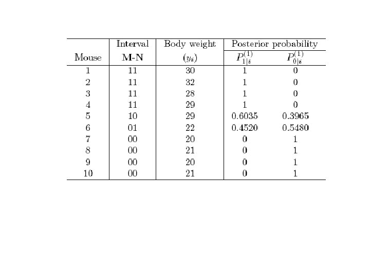
 M 1 1 184") Posterior prob. Sam- Height Marker genotype QTL ple (cm, y) M 1 1 184 (y 1) Mm (1) 2 185 (y 2) Mm (1) Nn (1) 1|2 0|2 3 180 (y 3) Mm (1) Nn (1) 1|3 0|3 4 182 (y 4) Mm (1) nn (0) 1|4 0|4 5 167 (y 5) mm (0) nn (0) 1|5 0|5 6 169 (y 6) mm (0) nn (0) 1|6 0|6 7 165 (y 7) mm (0) nn (0) 1|7 0|7 8 166 (y 8) mm (0) Nn (1) 1|8 0|8 M 2 Qq qq 1|1 0|1 Nn (1)
Posterior prob. Sam- Height Marker genotype QTL ple (cm, y) M 1 1 184 (y 1) Mm (1) 2 185 (y 2) Mm (1) Nn (1) 1|2 0|2 3 180 (y 3) Mm (1) Nn (1) 1|3 0|3 4 182 (y 4) Mm (1) nn (0) 1|4 0|4 5 167 (y 5) mm (0) nn (0) 1|5 0|5 6 169 (y 6) mm (0) nn (0) 1|6 0|6 7 165 (y 7) mm (0) nn (0) 1|7 0|7 8 166 (y 8) mm (0) Nn (1) 1|8 0|8 M 2 Qq qq 1|1 0|1 Nn (1)
 Give initiate values (0) = ( 1, 0, 2, )(0), (2)") EM algorithm (1) Give initiate values (0) = ( 1, 0, 2, )(0), (2) Calculate 1|i(1) and 0|i(1) using Eqs. 1 and 2, (3) Calculate (1) using 1|i(1) and 0|i(1), (4) Repeat (2) and (3) until convergence.
EM algorithm (1) Give initiate values (0) = ( 1, 0, 2, )(0), (2) Calculate 1|i(1) and 0|i(1) using Eqs. 1 and 2, (3) Calculate (1) using 1|i(1) and 0|i(1), (4) Repeat (2) and (3) until convergence.
 • • View as a") Two approaches for estimating the QTL position ( ) • • View as a variable being estimated (derive the log-likelihood equation for the MLE of ), View as a fixed parameter by assuming that the QTL is located at a particular position.
Two approaches for estimating the QTL position ( ) • • View as a variable being estimated (derive the log-likelihood equation for the MLE of ), View as a fixed parameter by assuming that the QTL is located at a particular position.
 test statistics H 0: There is no QTL ( 1= 0") Log-likelihood ratio (LR) test statistics H 0: There is no QTL ( 1= 0 or a* = 0) – reduced model H 1: There is a QTL ( 1 0 or a* 0) – full model Under H 0: L 0 = L(y, M|, a*=0, ) Under H 1: L 1 = L(y, M|^ 1, ^ 0, ^ 2, ) LR = -2(log L 0 – log L 1)
Log-likelihood ratio (LR) test statistics H 0: There is no QTL ( 1= 0 or a* = 0) – reduced model H 1: There is a QTL ( 1 0 or a* 0) – full model Under H 0: L 0 = L(y, M|, a*=0, ) Under H 1: L 1 = L(y, M|^ 1, ^ 0, ^ 2, ) LR = -2(log L 0 – log L 1)
 The profile of log-likelihood ratios across a linkage group LR Testing position
 The determination of thresholds Sample Original 1 1 2 3 4 5 6 7 8 Permutation 2 … 1000 184 165 x … x 185 182 x … x 180 169 x … x 182 167 x … x 167 185 x … x 169 180 x … x 165 166 x … x 166 184 x … x LR 1 LR 2 … LR 1000 M 1 M 2 QTL Mm (1) mm (0) Nn (1) nn (0) Nn (1) ? ? ? ? The critical value is the 95 th or 99 th percentiles of the 1000 LRs
 Result interpretations A poplar genome project Objectives: • Identify QTL affecting stemwood growth and production using molecular markers; • Develop fast-growing cultivars using marker-assisted selection
 euramerican") Materials and Methods • Poplar hybrids F 1 hybrids from eastern cottonwood (D) euramerican poplar (E) (a hybrid between eastern cottonwood black poplar) Four hundred fifty (450) F 1 hybrids were planted in a field trial • DNA extraction and marker arrays A total of 560 markers were detected from a subset of F 1 hybrids (90) • Genetic linkage map construction
Materials and Methods • Poplar hybrids F 1 hybrids from eastern cottonwood (D) euramerican poplar (E) (a hybrid between eastern cottonwood black poplar) Four hundred fifty (450) F 1 hybrids were planted in a field trial • DNA extraction and marker arrays A total of 560 markers were detected from a subset of F 1 hybrids (90) • Genetic linkage map construction
 Profile of the log-likelihood ratios across the length of a linkage group Critical value determined from permutation tests
 Advantages and disadvantages Compared with single marker analysis, interval mapping has several advantages: • The position of the QTL can be inferred by a support interval; • The estimated position and effects of the QTL tend to be asymptotically unbiased if there is only one segregating QTL on a chromosome; • The method requires fewer individuals than single marker analysis for the detection of QTL Disadvantages: • The test is not an interval test (a test that can distinguish whether or not there is a QTL within a defined interval and should be independent of the effects of QTL that are outside a defined region). • Even when there is no QTL within an interval, the likelihood profile on the interval can still exceed the threshold (ghost QTL) if there is QTL at some nearby region on the chromosome. • If there is more than one QTL on a chromosome, the test statistic at the position being tested will be affected by all QTL and the estimated positions and effects of “QTL” identified by this method are likely to be biased. • It is not efficient to use only two markers at a time for testing, since the information from other markers is not utilized.
 Limitations of single marker analysis Limitations") Composite Method for QTL Mapping Zeng (1993, 1994) Limitations of single marker analysis Limitations of interval mapping • The test statistic on one interval can be affected by QTL located at other intervals (not precise); • Only two markers are used at a time (not efficient) Strategies to overcome these limitations • Equally use all markers at a time (time consuming, model selection, test statistic) • One interval is analyzed using other markers to control genetic background
Composite Method for QTL Mapping Zeng (1993, 1994) Limitations of single marker analysis Limitations of interval mapping • The test statistic on one interval can be affected by QTL located at other intervals (not precise); • Only two markers are used at a time (not efficient) Strategies to overcome these limitations • Equally use all markers at a time (time consuming, model selection, test statistic) • One interval is analyzed using other markers to control genetic background
 Foundation of composite interval mapping • Interval mapping – Only use two flanking markers at a time to test the existence of a QTL (throughout the entire chromosome) • Composite interval mapping – Conditional on other markers, two flanking markers are used to test the existence of a QTL in a test interval Note: An understanding of the foundation of composite interval mapping needs a lot of basic statistics. Please refer to A. Stuart and J. K. Ord’s book, Kendall’s Advanced Theory of Statistics, 5 th Ed, Vol. 2. Oxford University Press, New York.
 Assume a backcross and one marker Aa × aa Aa aa Frequency ½ ½ “Value” 1 0 “Deviation” ½ -½ Variance 2 = (½)2×½ + (-½)2×½ = ¼ Mean 1 ½ Two markers, A and B: Aa. Bb × aabb Aa. Bb Aabb aa. Bb aabb Frequency ½(1 -r) ½r ½r ½(1 -r) “Value” (A) 1 1 0 0 “Value” (B) 1 0 1 0 Covariance AB = (1 -2 r)/4 Correlation = 1 - 2 r
 Conditional variance: 2 B|A = 2 B - 2 AB/ 2 A = ¼ - [(1 -2 r)/4]2/(¼) = r(1 -r) For general markers, j and k, we have Covariance jk = (1 - 2 rjk)/4 Correlation = 1 - 2 rjk Conditional variance: 2 k|j = 2 k - 2 kj / 2 j = ¼ - [(1 -2 rjk)/4]2/(¼) = rjk(1 -rjk)
 Three markers, j, k and l Covariance between markers j and k conditional on marker l: jk|l= jk - jl kl / 2 l = [(1 -2 rjk)-(1 -2 rjl)(1 -2 rkl)]/4 = 0 For order -j-l-k- or -k -l-j rkl(1 -rkl)(1 -2 rjk) For order -j-k-l- or -l-k-j rjl(1 -rjl)(1 -2 rjk) For order -l-j-k- or -k-j-l Note: (1 -2 rjk)=(1 -2 rjl)(1 -2 rkl) for order jlk or klj
 Three markers, j, k and l Variance of markers j conditional on markers k and l 2 j|kl = 2 j|k - 2 jl|k / 2 l|k = 2 j|l - 2 jk|l / 2 k|l = 2 j|k For order -j-k-l 2 j|l For order -k-l-j [rkj(1 -rkj)rjl(1 -rjl)]/[rkl(1 -rkl)] For order -k-j-l. In general, the variance of markers j conditional on all other markers is 2 j|s_ = 2 j|(j-1)(j+1) , s_ is denotes a set that includes all markers except marker j.
 Important conclusions: · Conditional on an intermediate marker, the covariance between two flanking markers is expected to be zero. · This conclusion is the foundation for composite interval mapping which aims to eliminate the effect of genome background on the estimation of QTL parameters
 Four markers, j < k, l < m Covariance between markers j and k conditional on markers l and m: jk|lm = jk|l – jm|l km|l / 2 m|l = jk|m – jl|m kl|m / 2 l|m = 0 For order -j-l-k-m- or -j-m-k-l jk|l For order -j-k-l-m jk|m For order -l-m-j-k [rlj(1 - rlj)rkm(1 - rkm)(1 - 2 rjk)]/[rlm(1 - rlm)] For order -l-j-k-m-
-l-j-k-m-(m+1)-, we have jk|(l-1)lm(m+1) = jk|lm, which says that The covariance") In general, for -(l-1)-l-j-k-m-(m+1)-, we have jk|(l-1)lm(m+1) = jk|lm, which says that The covariance between markers j and (j+1) conditional on all other markers is j(j+1)|s_ = j(j+1)|(j-1)(j+2) (s_ is denotes a set that includes all markers except markers j and (j+1).
In general, for -(l-1)-l-j-k-m-(m+1)-, we have jk|(l-1)lm(m+1) = jk|lm, which says that The covariance between markers j and (j+1) conditional on all other markers is j(j+1)|s_ = j(j+1)|(j-1)(j+2) (s_ is denotes a set that includes all markers except markers j and (j+1).
 Marker and QTL Assume a backcross and one QTL Qq x qq Qq + qq Frequency ½ Value a 0 Variance 2 = 1/4 a 2 One marker A and one QTL u: Aa. Qq x aaqq Aa. Qq Aaqq Frequency ½(1 -r) ½r Value (A) 1 1 Value (Q) a 0 Covariance ku = (1 -2 ruk)a/4 Correlation = 1 -2 rku mean ½ ½a aa. Qq ½r 0 a aaqq ½(1 -r) 0 0
 Two markers, j and k, and one trait, y, including many QTLs Covariance between trait y and marker j conditional on marker k yj|k = yj - yk jk / 2 k = u=1[(1 -2 ruj)-(1 -2 ruk)(1 -2 rjk)]au/4 = rjk(1 -rjk) u j(1 -2 ruj)au + j
 Covariance between trait y and marker j conditional on markers k and l yj|kl = yj/k - yk/j jl/k / 2 l/k = yj/l - yk/l jk/l / 2 k/l = yj/k For order -j-k-l yj/l For order -j-l-k[rjk(1 - rjk)]/[rlk(1 - rlk)] l
-j-(j+1)-…-, we have yj|s_ = yj|(j-1)(j+1) Partial regression coefficient byj|s_") In general, for order -…-(j-1)-j-(j+1)-…-, we have yj|s_ = yj|(j-1)(j+1) Partial regression coefficient byj|s_ = yj|s_/ 2 j|s_ = yj|(j-1)(j+1)/ 2 j|(j-1)(j+1) = (j-1)
In general, for order -…-(j-1)-j-(j+1)-…-, we have yj|s_ = yj|(j-1)(j+1) Partial regression coefficient byj|s_ = yj|s_/ 2 j|s_ = yj|(j-1)(j+1)/ 2 j|(j-1)(j+1) = (j-1)
") Two summations: • • The first is for all QTL located between markers (j-1) and j The second is for all QTL located between markers j and (j+1).
Two summations: • • The first is for all QTL located between markers (j-1) and j The second is for all QTL located between markers j and (j+1).
 Important conclusion: The partial regression coefficient depends only on those QTL which are located between markers (j-1) and (j+1)
![Suppose there is only one QTL [between markers (j-1) and j], we have byj|s_](https://present5.com/presentation/317f9338536ed2f71ada6b59ddf986ae/image-74.jpg "Suppose there is only one QTL [between markers (j-1) and j], we have byj|s_") Suppose there is only one QTL [between markers (j-1) and j], we have byj|s_ = [r(j-1)u(1 - r(j-1)u)(1 - 2 ruj)]/[r(j-1)j(1 - r(j 1)j)]au. An estimate of byj|s_ is a biased estimate of au.
Suppose there is only one QTL [between markers (j-1) and j], we have byj|s_ = [r(j-1)u(1 - r(j-1)u)(1 - 2 ruj)]/[r(j-1)j(1 - r(j 1)j)]au. An estimate of byj|s_ is a biased estimate of au.
 Properties of composite interval mapping • In the multiple regression analysis, assuming additivity of QTL effects between loci (i. e. , ignoring interactions), the expected partial regression coefficient of the trait on a marker depends only on those QTL which are located on the interval bracketed by the two neighboring markers, and is unaffected by the effects of QTL located on other intervals. • Conditioning on unlinked markers in the multiple regression analysis will reduce the sampling variance of the test statistic by controlling some residual genetic variation and thus will increase the power of QTL mapping.
 • Conditioning on linked markers in the multiple regression analysis will reduce the chance of interference of possible multiple linked QTL on hypothesis testing and parameter estimation, but with a possible increase of sampling variance. • Two sample partial regression coefficients of the trait value on two markers in a multiple regression analysis are generally uncorrelated unless the two markers are adjacent markers.
 Composite model for interval mapping and regression analysis m-2 b zi: QTL genotype i xik: marker genotype yi = + a* zi + k kxik + e Expected means: Qq: + a* + kbkxik = a* + Xi. B qq: + kbkxik = Xi. B Xi = (1, xi 2, …, xi(m-2))1 x(m-1) M x 1 1 M 1 m 1 1 B = ( , b 1, b 2, …, bm-2)T M 1 m 1 0 +b 1
![Likelihood function L(y, M| ) = i=1 n[ 1|if 1(yi) + 0|if 0(yi)] log](https://present5.com/presentation/317f9338536ed2f71ada6b59ddf986ae/image-78.jpg "Likelihood function L(y, M| ) = i=1 n[ 1|if 1(yi) + 0|if 0(yi)] log") Likelihood function L(y, M| ) = i=1 n[ 1|if 1(yi) + 0|if 0(yi)] log L(y, M| ) = i=1 n log[ 1|if 1(yi) + 0|if 0(yi)] f 1(yi) = 1/[(2 )½ ]exp[-½(y- 1)2], 1= a*+Xi. B f 0(yi) = 1/[(2 )½ ]exp[-½(y- 0)2], 0= Xi. B Define 1|i = 1|if 1(yi)/[ 1|if 1(yi) + 0|if 0(yi)] 0|i = 0|if 1(yi)/[ 1|if 1(yi) + 0|if 0(yi)] (1) (2)
Likelihood function L(y, M| ) = i=1 n[ 1|if 1(yi) + 0|if 0(yi)] log L(y, M| ) = i=1 n log[ 1|if 1(yi) + 0|if 0(yi)] f 1(yi) = 1/[(2 )½ ]exp[-½(y- 1)2], 1= a*+Xi. B f 0(yi) = 1/[(2 )½ ]exp[-½(y- 0)2], 0= Xi. B Define 1|i = 1|if 1(yi)/[ 1|if 1(yi) + 0|if 0(yi)] 0|i = 0|if 1(yi)/[ 1|if 1(yi) + 0|if 0(yi)] (1) (2)
/ i=1 n 1|i = 1 (Y-XB)´/c (3) B") a* = i=1 n 1|i(yi-a*-Xi. B)/ i=1 n 1|i = 1 (Y-XB)´/c (3) B = (X´X)-1 X´(Y- 1 a*) (4) 2 = 1/n (Y-XB)´(Y-XB) – a*2 c (5) = ( i=1 n 2 1|i + i=1 n 3 0|i)/(n 2+n 3) (6) Y = {yi}nx 1, = { 1|i}nx 1, c = i=1 n 1|i
a* = i=1 n 1|i(yi-a*-Xi. B)/ i=1 n 1|i = 1 (Y-XB)´/c (3) B = (X´X)-1 X´(Y- 1 a*) (4) 2 = 1/n (Y-XB)´(Y-XB) – a*2 c (5) = ( i=1 n 2 1|i + i=1 n 3 0|i)/(n 2+n 3) (6) Y = {yi}nx 1, = { 1|i}nx 1, c = i=1 n 1|i
 Hypothesis test H 0: a*=0 vs H 1: a* 0 L 0 = i=1 nf(yi) B = (X´X)-1 X´Y, 2=1/n(Y-XB)´(Y-XB) L 1= i=1 n[ 1|if 1(yi) + 0|if 0(yi)] LR = -2(ln. L 0 – ln. L 1) LOD = log. L 1 – log. L 0
 Example Interval mapping Composite interval mapping LR Testing position