Project Analysis Decision Making Engineering 90 Dr

Project Analysis / Decision Making Engineering 90 Dr. Gregory Crawford

Four Ways to do Project Analysis • Statistical / Regression Analysis (forecasting) • Sensitivity Analysis • Monte Carlo Simulations • Decision Trees Decision Tree

What’s the difference? Each shows a manager different aspects of the decision he/she faces: • Regression / Statistical Forecasting is a way to estimate future sales growth based on current or past performances. • Sensitivity Analysis shows her how much each variable affects the NPV. • Monte Carlo gives a statistical breakdown of the possible outcomes. • Decision Trees are visual representations of the average outcome.

Regression and Statistical Forecasting • Mathematically model past sales of either same product or similar product • Projects future sales as a function of these past sales with respect to time We will talk about two types of regression • Linear Regression • Polynomial Regression (but there are many more, logarithmic, exponential, etc)

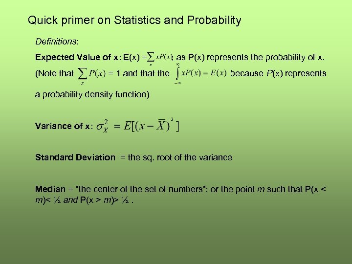Quick primer on Statistics and Probability Definitions: Expected Value of x: E(x) = ; as P(x) represents the probability of x. (Note that = 1 and that the because P(x) represents a probability density function) Variance of x: Standard Deviation = the sq. root of the variance Median = “the center of the set of numbers”; or the point m such that P(x < m)< ½ and P(x > m)> ½.

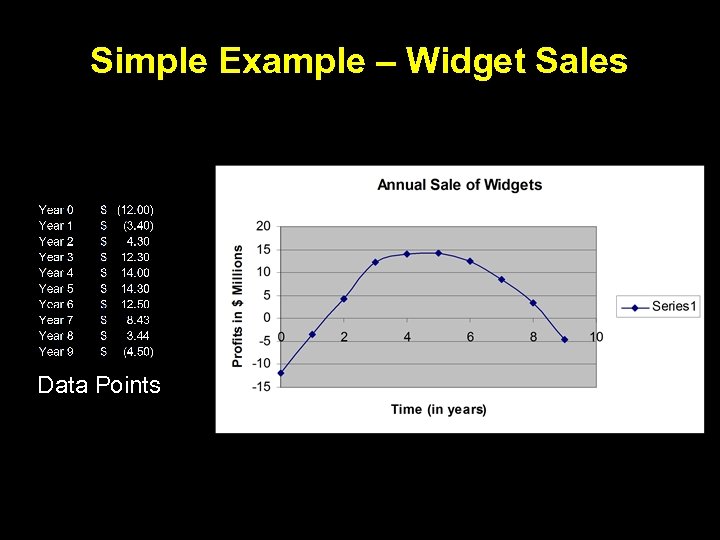Simple Example – Widget Sales Data Points

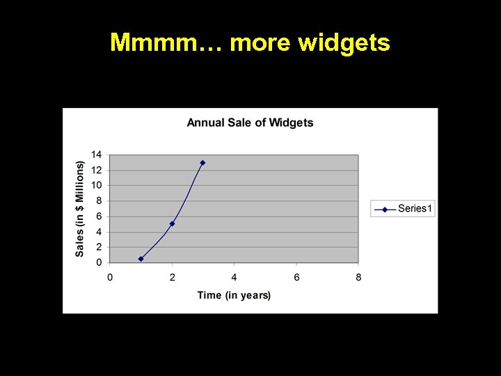
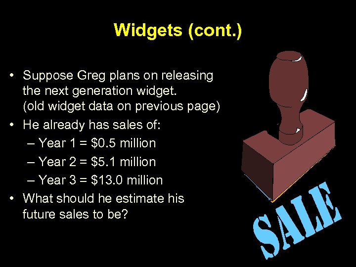Widgets (cont. ) • Suppose Greg plans on releasing the next generation widget. (old widget data on previous page) • He already has sales of: – Year 1 = $0. 5 million – Year 2 = $5. 1 million – Year 3 = $13. 0 million • What should he estimate his future sales to be?

Mmmm… more widgets

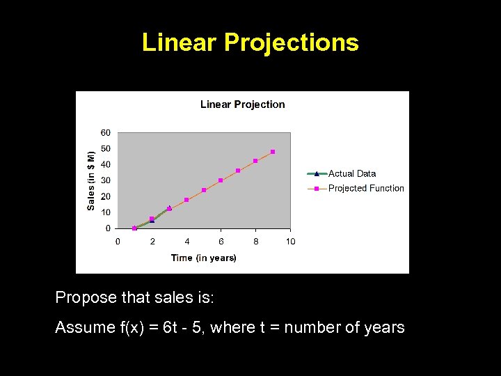Linear Projections Propose that sales is: Assume f(x) = 6 t - 5, where t = number of years

Regression – Least Squares • Is there a formal way to get this estimation function? • Fit a line such that the square of the vertical deviations between the function and the data points is minimized

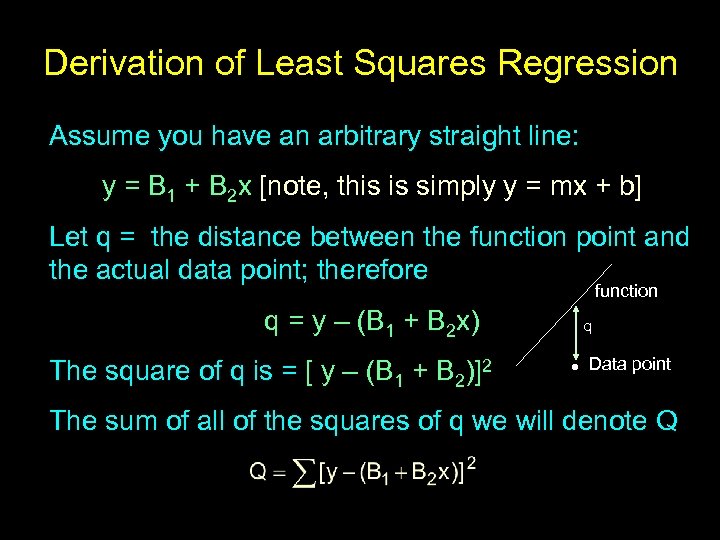Derivation of Least Squares Regression Assume you have an arbitrary straight line: y = B 1 + B 2 x [note, this is simply y = mx + b] Let q = the distance between the function point and the actual data point; therefore function q = y – (B 1 + B 2 x) The square of q is = [ y – (B 1 + B 2)]2 q • Data point The sum of all of the squares of q we will denote Q

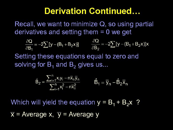Derivation Continued… Recall, we want to minimize Q, so using partial derivatives and setting them = 0 we get Setting these equations equal to zero and solving for B 1 and B 2 gives us. . . Which will yield the equation y = B 1 + B 2 x ? x = Average x, y = Average y

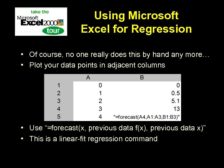Using Microsoft Excel for Regression • Of course, no one really does this by hand any more… • Plot your data points in adjacent columns • Use “=forecast(x, previous data f(x), previous data x)” • This is a linear-fit regression command

What’s wrong with this picture? • First, it is unrealistic to have infinitely rising sales • Second, it doesn’t fit with Greg’s previous widget product’s sales, which eventually decline • Let’s try to find a function that takes the first set of widget sales into account.

F(x) = ax 2 + bx + c New function data In fact, the function is f(x) = -. 8(x-4)2 + 13

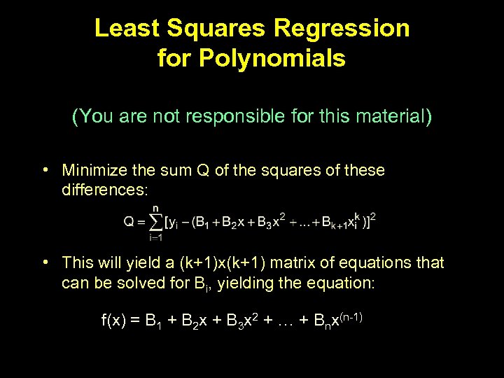Least Squares Regression for Polynomials (You are not responsible for this material) • Minimize the sum Q of the squares of these differences: • This will yield a (k+1)x(k+1) matrix of equations that can be solved for Bi, yielding the equation: f(x) = B 1 + B 2 x + B 3 x 2 + … + Bnx(n-1)

Summary • Least squares regression is a common scientific & engineering practice. • In business, it can be used to forecast possible future trends. • You’re responsible for linear least squares regression only.

Sensitivity Analysis • Set up an Excel spreadsheet that will calculate your projects NPV • Individually change your assumptions to see how the NPV changes with respect to different variables • Helps to determine how much to spend on additional information

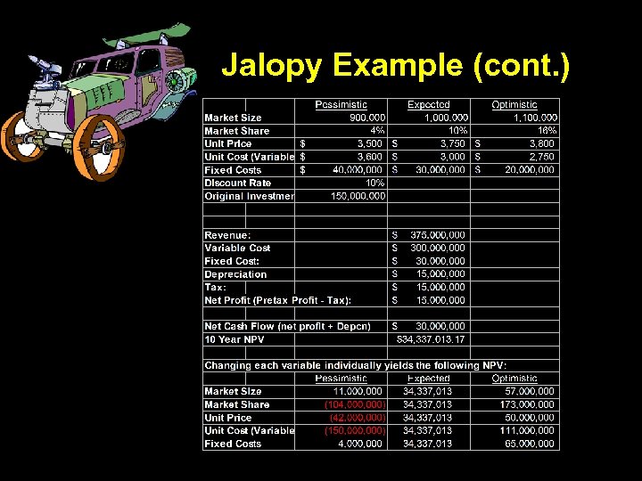
Jalopy Motor’s Example Suppose that you forecast the following for an electric scooter project: • Market Size of. 9 (worst case)– 1. 1 million (best case) customers • Market Share of between 4% (wc)and 16% (bc) after the first year • Unit price between $3, 500 (wc) and $3, 800 (bc) • Unit cost (variable) between $3, 600 (wc) and $2, 750 (bc) • Fixed costs between $40 (wc) and 20 million (bc). From Principles of Corporate Finance, (c) 1996 Brealey/Myers

Jalopy Example (cont. )

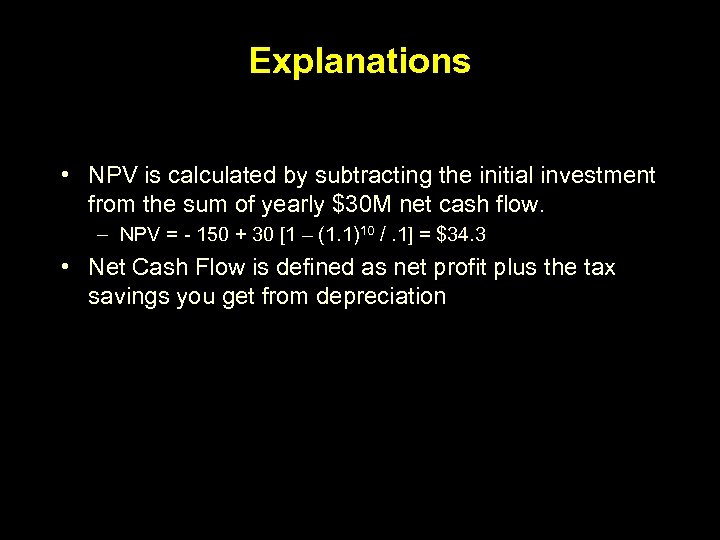Explanations • NPV is calculated by subtracting the initial investment from the sum of yearly $30 M net cash flow. – NPV = - 150 + 30 [1 – (1. 1)10 /. 1] = $34. 3 • Net Cash Flow is defined as net profit plus the tax savings you get from depreciation

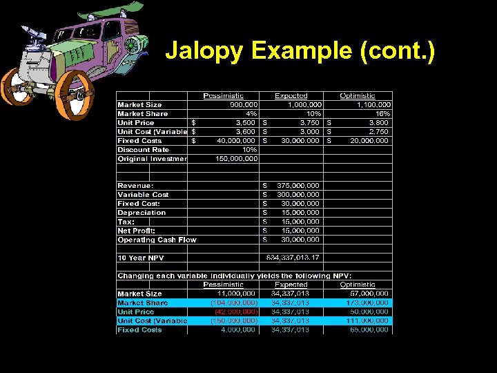Jalopy Example (cont. )

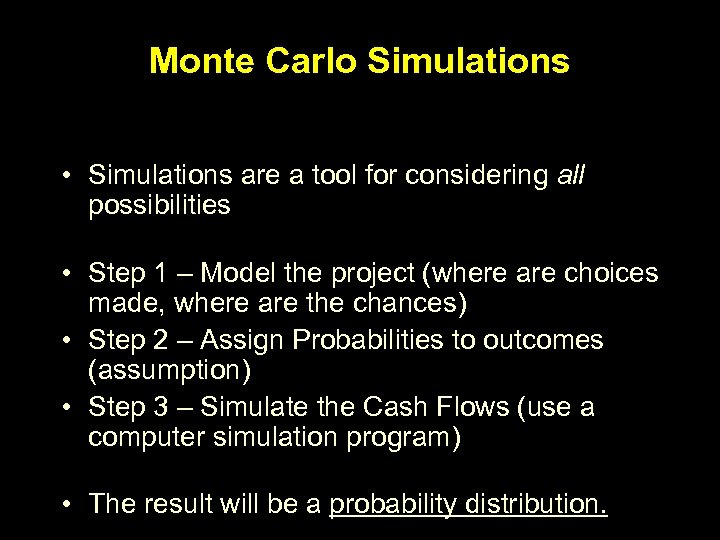Monte Carlo Simulations • Simulations are a tool for considering all possibilities • Step 1 – Model the project (where are choices made, where are the chances) • Step 2 – Assign Probabilities to outcomes (assumption) • Step 3 – Simulate the Cash Flows (use a computer simulation program) • The result will be a probability distribution.

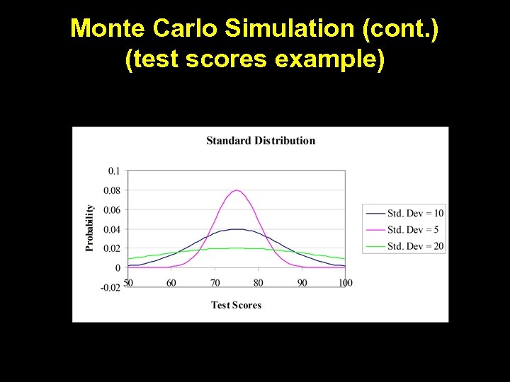Monte Carlo Simulation (cont. ) (test scores example)

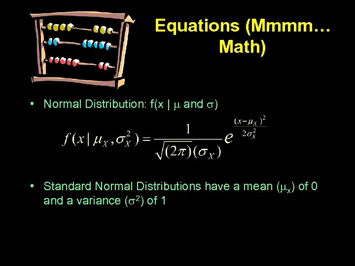Equations (Mmmm… Math) • Normal Distribution: f(x | and ) • Standard Normal Distributions have a mean ( x) of 0 and a variance ( 2) of 1

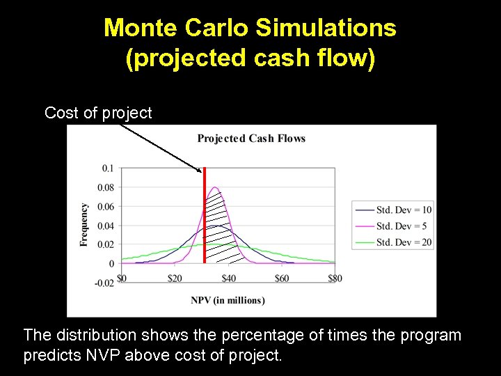Monte Carlo Simulations (projected cash flow) Cost of project The distribution shows the percentage of times the program predicts NVP above cost of project.

Summary Monte Carlo • You are not responsible for this on the test. • Statistical breakdown of possible outcomes. • Dealing with continuous distribution.

What is a Decision Tree? • A Visual Representation of Choices, Consequences, Probabilities, and Opportunities. • A Way of Breaking Down Complicated Situations Down to Easier-to-Understand Scenarios. Decision Tree

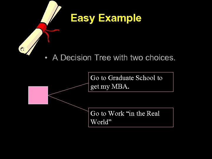Easy Example • A Decision Tree with two choices. Go to Graduate School to get my MBA. Go to Work “in the Real World”

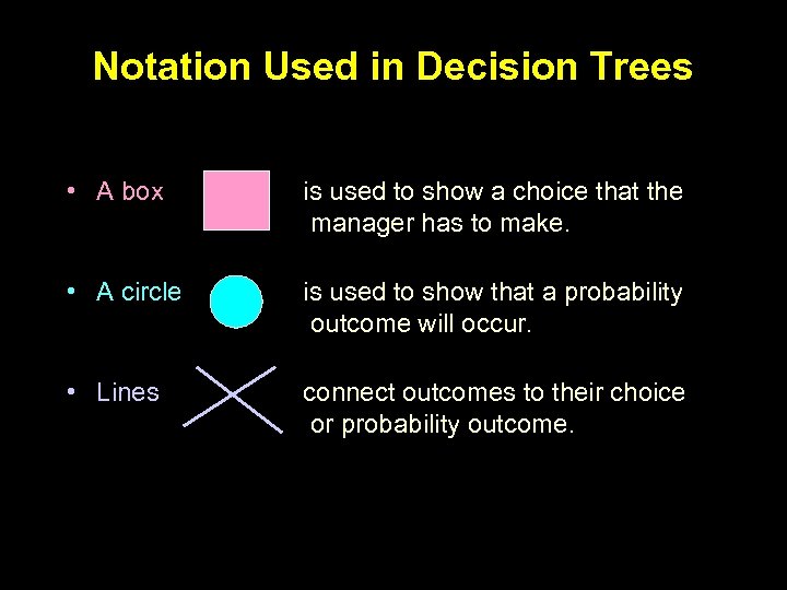Notation Used in Decision Trees • A box is used to show a choice that the manager has to make. • A circle is used to show that a probability outcome will occur. • Lines connect outcomes to their choice or probability outcome.

Easy Example - Revisited What are some of the costs we should take into account when deciding whether or not to go to business school? • Tuition and Fees • Rent / Food / etc. • Opportunity cost of salary • Anticipated future earnings

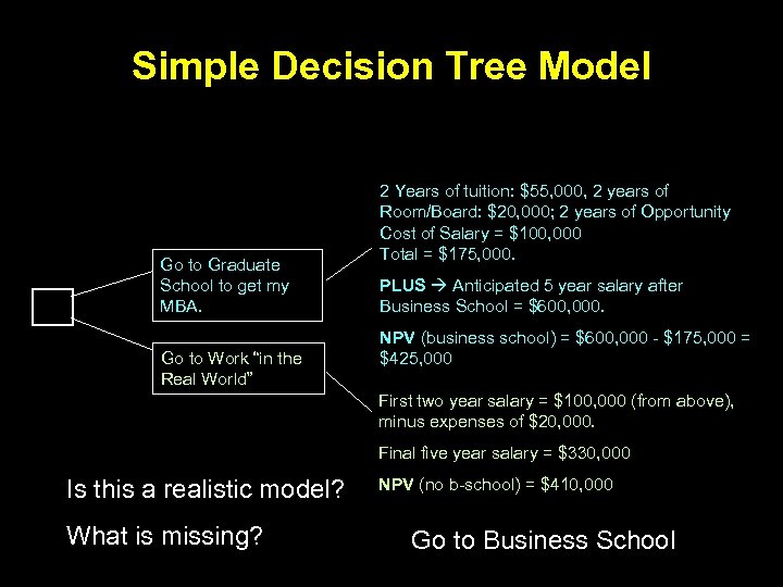Simple Decision Tree Model Go to Graduate School to get my MBA. Go to Work “in the Real World” 2 Years of tuition: $55, 000, 2 years of Room/Board: $20, 000; 2 years of Opportunity Cost of Salary = $100, 000 Total = $175, 000. PLUS Anticipated 5 year salary after Business School = $600, 000. NPV (business school) = $600, 000 - $175, 000 = $425, 000 First two year salary = $100, 000 (from above), minus expenses of $20, 000. Final five year salary = $330, 000 Is this a realistic model? What is missing? NPV (no b-school) = $410, 000 Go to Business School

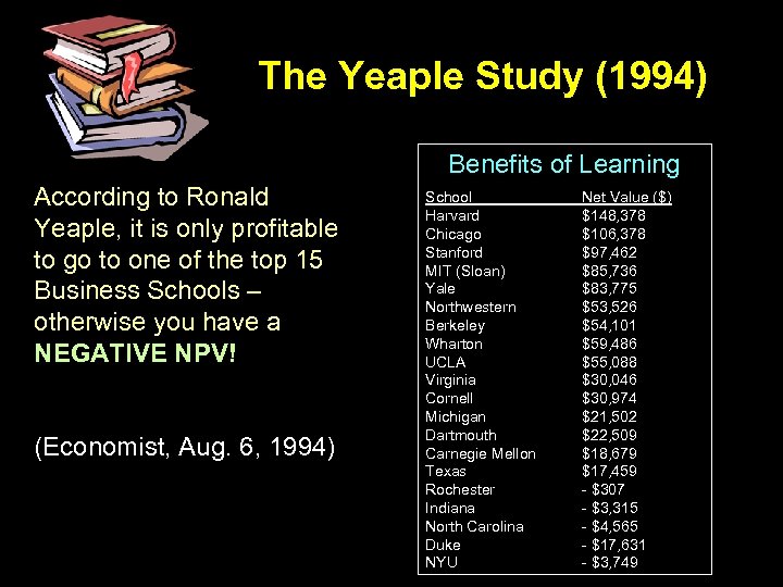The Yeaple Study (1994) Benefits of Learning According to Ronald Yeaple, it is only profitable to go to one of the top 15 Business Schools – otherwise you have a NEGATIVE NPV! (Economist, Aug. 6, 1994) School Harvard Chicago Stanford MIT (Sloan) Yale Northwestern Berkeley Wharton UCLA Virginia Cornell Michigan Dartmouth Carnegie Mellon Texas Rochester Indiana North Carolina Duke NYU Net Value ($) $148, 378 $106, 378 $97, 462 $85, 736 $83, 775 $53, 526 $54, 101 $59, 486 $55, 088 $30, 046 $30, 974 $21, 502 $22, 509 $18, 679 $17, 459 - $307 - $3, 315 - $4, 565 - $17, 631 - $3, 749

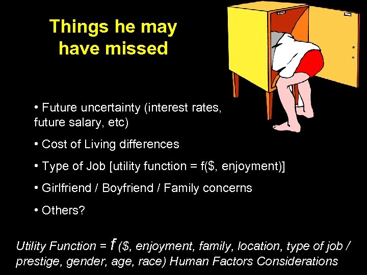Things he may have missed • Future uncertainty (interest rates, future salary, etc) • Cost of Living differences • Type of Job [utility function = f($, enjoyment)] • Girlfriend / Boyfriend / Family concerns • Others? Utility Function = f ($, enjoyment, family, location, type of job / prestige, gender, age, race) Human Factors Considerations

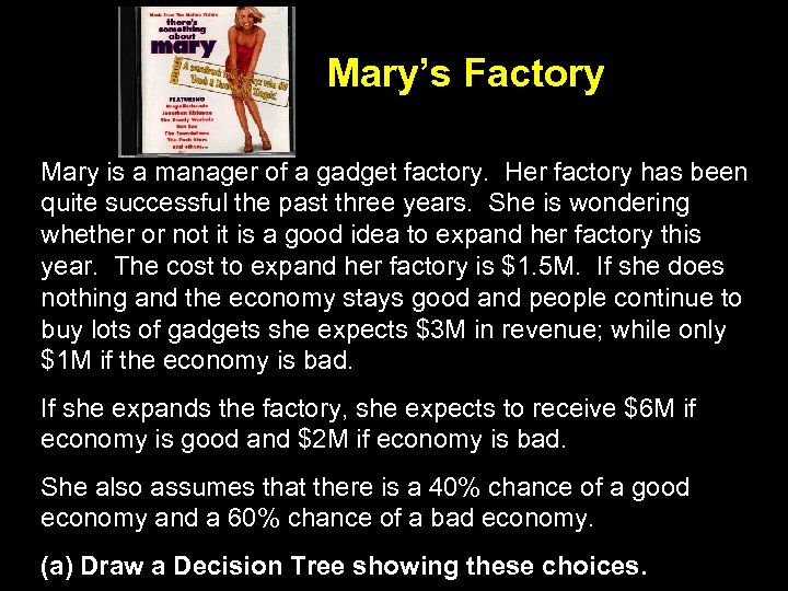Mary’s Factory Mary is a manager of a gadget factory. Her factory has been quite successful the past three years. She is wondering whether or not it is a good idea to expand her factory this year. The cost to expand her factory is $1. 5 M. If she does nothing and the economy stays good and people continue to buy lots of gadgets she expects $3 M in revenue; while only $1 M if the economy is bad. If she expands the factory, she expects to receive $6 M if economy is good and $2 M if economy is bad. She also assumes that there is a 40% chance of a good economy and a 60% chance of a bad economy. (a) Draw a Decision Tree showing these choices.

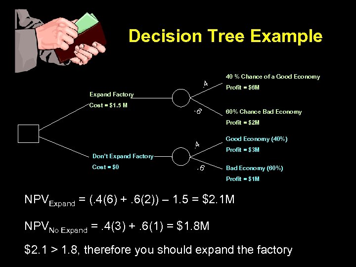Decision Tree Example. 4 40 % Chance of a Good Economy Profit = $6 M Expand Factory Cost = $1. 5 M . 6 60% Chance Bad Economy Profit = $2 M . 4 Don’t Expand Factory Cost = $0 . 6 Good Economy (40%) Profit = $3 M Bad Economy (60%) Profit = $1 M NPVExpand = (. 4(6) +. 6(2)) – 1. 5 = $2. 1 M NPVNo Expand =. 4(3) +. 6(1) = $1. 8 M $2. 1 > 1. 8, therefore you should expand the factory

Example 2 – Joe’s Garage Joe’s garage is considering hiring another mechanic. The mechanic would cost them an additional $50, 000 / year in salary and benefits. If there a lot of accidents in Providence this year, they anticipate making an additional $75, 000 in net revenue. If there are not a lot of accidents, they could lose $20, 000 off of last year’s total net revenues. Because of all the ice on the roads, Joe thinks that there will be a 70% chance of “a lot of accidents” and a 30% chance of “fewer accidents”. Assume if he doesn’t expand he will have the same revenue as last year. Draw a decision tree for Joe and tell him what he should do.

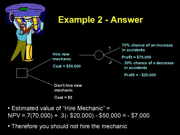Example 2 - Answer. 7 Hire new mechanic Cost = $50, 000 70% chance of an increase in accidents . 3 Profit = $70, 000 30% chance of a decrease in accidents Profit = - $20, 000 Don’t hire new mechanic Cost = $0 • Estimated value of “Hire Mechanic” = NPV =. 7(70, 000) +. 3(- $20, 000) - $50, 000 = - $7, 000 • Therefore you should not hire the mechanic

Mary’s Factory – With Options A few days later she was told that if she expands, she can opt to either (a) expand the factory further if the economy is good which costs 1. 5 M, but will yield an additional $2 M in profit when economy is good but only $1 M when economy is bad, (b) abandon the project and sell the equipment she originally bought for $1. 3 M, or (c) do nothing. (b) Draw a decision tree to show these three options for each possible outcome, and compute the NPV for the expansion.

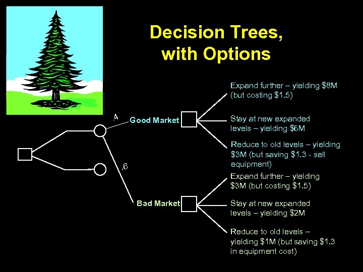Decision Trees, with Options Expand further – yielding $8 M (but costing $1. 5) . 4 Good Market Stay at new expanded levels – yielding $6 M Reduce to old levels – yielding $3 M (but saving $1. 3 - sell equipment) . 6 Expand further – yielding $3 M (but costing $1. 5) Bad Market Stay at new expanded levels – yielding $2 M Reduce to old levels – yielding $1 M (but saving $1. 3 in equipment cost)

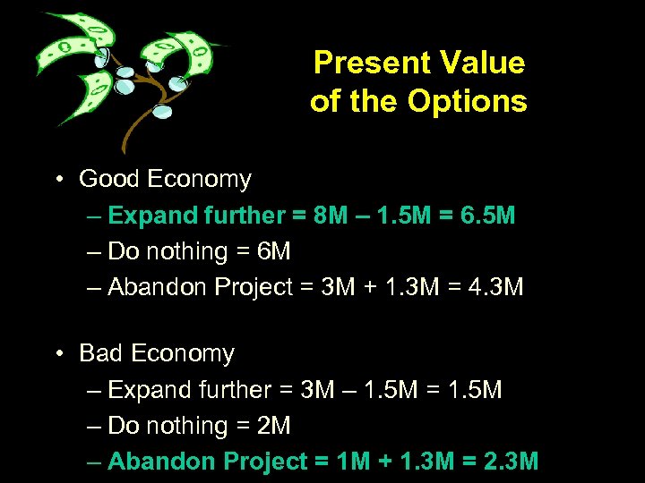Present Value of the Options • Good Economy – Expand further = 8 M – 1. 5 M = 6. 5 M – Do nothing = 6 M – Abandon Project = 3 M + 1. 3 M = 4. 3 M • Bad Economy – Expand further = 3 M – 1. 5 M = 1. 5 M – Do nothing = 2 M – Abandon Project = 1 M + 1. 3 M = 2. 3 M

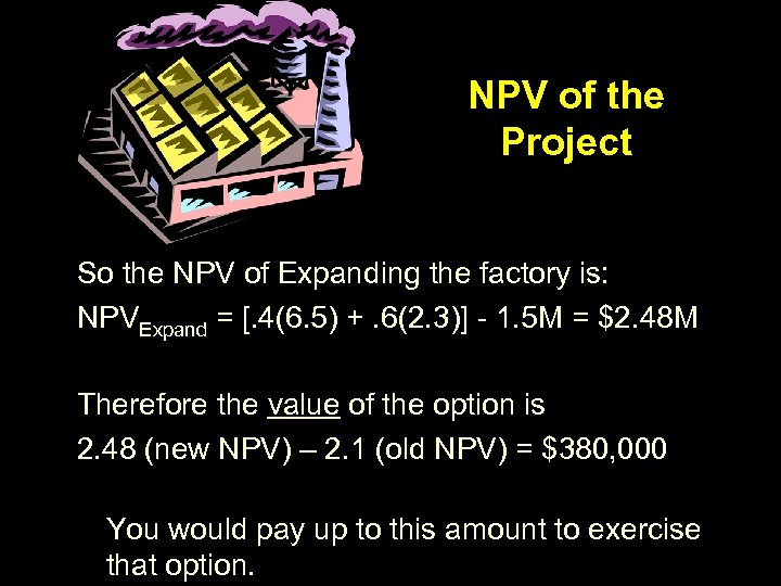NPV of the Project So the NPV of Expanding the factory is: NPVExpand = [. 4(6. 5) +. 6(2. 3)] - 1. 5 M = $2. 48 M Therefore the value of the option is 2. 48 (new NPV) – 2. 1 (old NPV) = $380, 000 You would pay up to this amount to exercise that option.

Mary’s Factory – Discounting Before Mary takes this to her boss, she wants to account for the time value of money. The gadget company uses a 10% discount rate. The cost of expanding the factory is borne in year zero but the revenue streams are in year one. (c) Compute the NPV in part (a) again, this time account the time value of money in your analysis. Should she expand the factory?

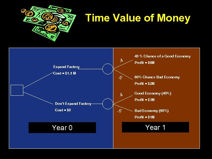Time Value of Money . 4 40 % Chance of a Good Economy Profit = $6 M Expand Factory Cost = $1. 5 M . 6 60% Chance Bad Economy Profit = $2 M . 4 Don’t Expand Factory Cost = $0 . 6 Good Economy (40%) Profit = $3 M Bad Economy (60%) Profit = $1 M Year 0 Year 1

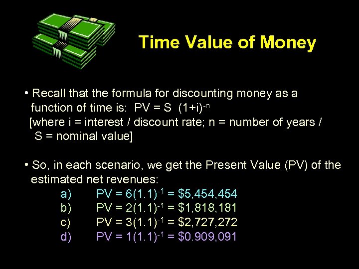Time Value of Money • Recall that the formula for discounting money as a function of time is: PV = S (1+i)-n [where i = interest / discount rate; n = number of years / S = nominal value] • So, in each scenario, we get the Present Value (PV) of the estimated net revenues: a) PV = 6(1. 1)-1 = $5, 454 b) PV = 2(1. 1)-1 = $1, 818, 181 c) PV = 3(1. 1)-1 = $2, 727, 272 d) PV = 1(1. 1)-1 = $0. 909, 091

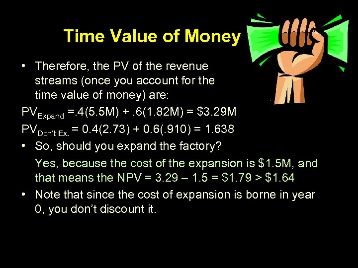Time Value of Money • Therefore, the PV of the revenue streams (once you account for the time value of money) are: PVExpand =. 4(5. 5 M) +. 6(1. 82 M) = $3. 29 M PVDon’t Ex. = 0. 4(2. 73) + 0. 6(. 910) = 1. 638 • So, should you expand the factory? Yes, because the cost of the expansion is $1. 5 M, and that means the NPV = 3. 29 – 1. 5 = $1. 79 > $1. 64 • Note that since the cost of expansion is borne in year 0, you don’t discount it.

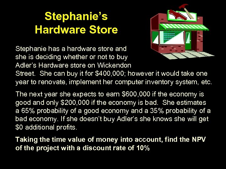Stephanie’s Hardware Store Stephanie has a hardware store and she is deciding whether or not to buy Adler’s Hardware store on Wickendon Street. She can buy it for $400, 000; however it would take one year to renovate, implement her computer inventory system, etc. The next year she expects to earn $600, 000 if the economy is good and only $200, 000 if the economy is bad. She estimates a 65% probability of a good economy and a 35% probability of a bad economy. If she doesn’t buy Adler’s she knows she will get $0 additional profits. Taking the time value of money into account, find the NPV of the project with a discount rate of 10%

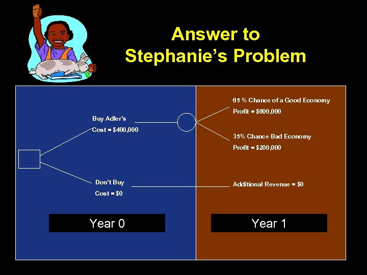Answer to Stephanie’s Problem 65 % Chance of a Good Economy Profit = $600, 000 Buy Adler’s Cost = $400, 000 35% Chance Bad Economy Profit = $200, 000 Don’t Buy Additional Revenue = $0 Cost = $0 Year 1

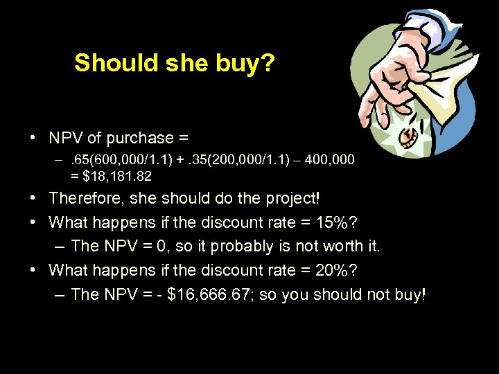Should she buy? • NPV of purchase = –. 65(600, 000/1. 1) +. 35(200, 000/1. 1) – 400, 000 = $18, 181. 82 • Therefore, she should do the project! • What happens if the discount rate = 15%? – The NPV = 0, so it probably is not worth it. • What happens if the discount rate = 20%? – The NPV = - $16, 666. 67; so you should not buy!