6e88486075749c3693f797db2e3e2c2a.ppt
- Количество слайдов: 40
Processing, Analyzing, and Displaying Functional MRI Data Robert W Cox, Ph. D SSCC / NIMH / NIH / DHHS / USA / EARTH BRCP Hawaii 2004
Shocking Truths about FMRI ! • Goal: Find and Characterize Neural Goal • “Activations” (whatever that means) Shocking Revelation #1: #1 FMRI data are (mostly) crap • But: All other neuroimaging data are, too Þ You must know what you are doing! • Shocking Revelation #2: #2 Most FMRI papers are weak on analysis 2
Points to Ponder & Discuss • • Field has relatively poor understanding of physiological and physics issues underlying fluctuations (both “signal” and “noise”) in FMRI time series in living brain tissue Virtually all FMRI studies are of groups • Categorizing individuals (phenotyping) is HARD • Combining & contrasting multiple human brains is non-trivial (e. g. , align anatomies? how well? ) • • Deciding what is “significant” is tricky Visualizing high-dimensional results at each voxel in 3 D space needs more work 3
Caveats and Disclaimers • Almost everything herein has an exception or complication • or is also the subject of ongoing research • Special types of data or stimuli may require special analysis tools • e. g. , perfusion-weighted FMRI (via arterial spin labeling) • non-repeatable tasks (e. g. , drug challenge) • Special types of questions may require special data and analyses • e. g. , relative timing of neural events 4
FMRI Data Acquisition & Theory • • FMRI data = scan subject’s brain rapidly (2 -3 s) and repeatedly (5 -100 min) • Speed relatively low spatial resolution (usually) Images are sensitized to T 2* = sensitive to magnetic field perturbations on sub-voxel scale • bigger perturbations image intensity is smaller • De-oxygenated hemoglobin perturbs magnetic field • Result: FMRI time series in each voxel measures Result how much deoxy. HB is present in that voxel • Observation: less deoxy. HB more neural activity Observation • Look for signal increases correlated with tasks • BOLD = Blood Oxygenation Level Dependent imaging 5
• • Meta-Method for Data Analysis Develop a mathematical model relating what we know stimulus timing, behavioral measurements, image data, to what we want to know location, amount, timing of neural activity Given data, use model to solve for unknown parameters in the neural activity (e. g. , when, where, how much) • Test for statistical significance, for each task and contrasts between tasks, in individuals and groups 6
Why FMRI Analysis Is Hard • Don’t know the true relation between neural “activity” and measurable MRI signal • What is neural “activity”, anyway? • What is connection between neural “activity” and hemodynamics and MRI signal? • Noise in time series data from living subjects is also poorly characterized • Makes statistical assessment hard • Result: There are many “reasonable” ways to Result do FMRI data analysis • And no good way to judge which are “better” 7
Temporal Models: Linear Convolution • Central Assumption: Assumption • FMRI (hemodynamic) response to 2 separated-in-time activations in same voxel is the separated-in-time sum of 2 copies of some individual task/stimulus response function The FMRI response to a single activation is called the hemodynamic response function (HRF) HRF 9
FMRI Data Analysis • Fit data time series in each voxel to a model derived from the HRF • Model is based on stimulus/task timing and on empirical models of the FMRI signal Simple HRF model: response to one brief stimulus 10
• Linearity of Response Multiple activation cycles in a voxel: • Assume that overlapping responses add • Result = convolution of HRF with task timing • Linearity is a good assumption • But not perfect — about 90% correct • Nevertheless, is widely taken to be true and is the basis for the “general linear model” (GLM) in FMRI analyses 3 Brief Activations 11
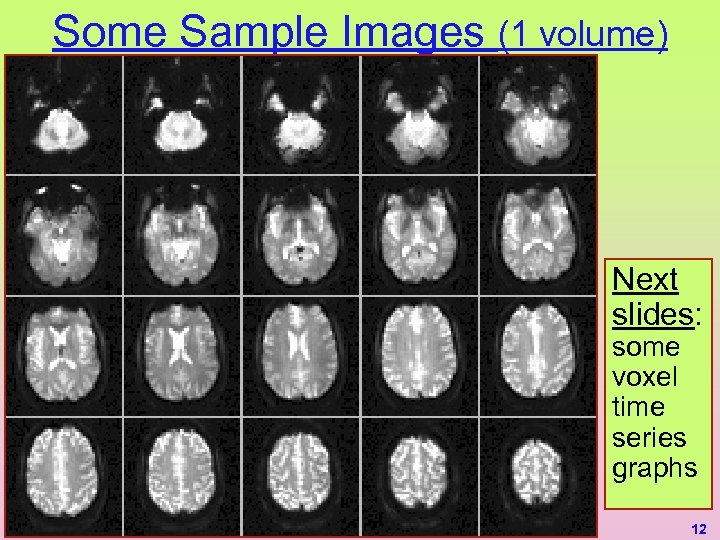
Some Sample Images (1 volume) Next slides: some voxel time series graphs 12
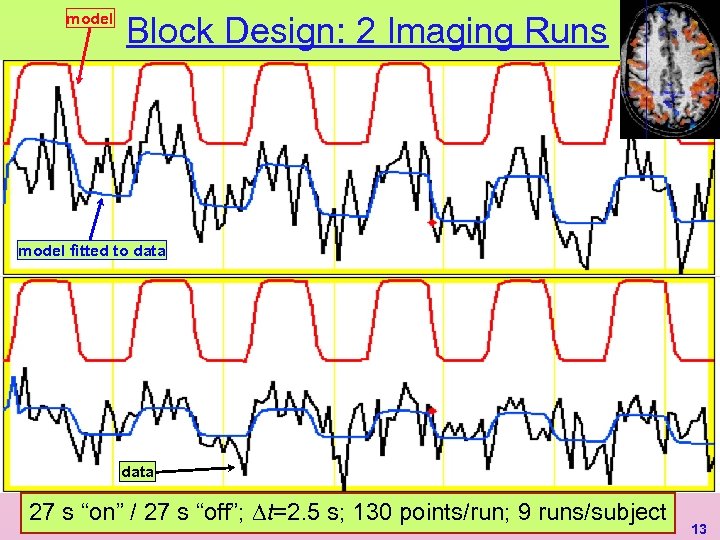
model Block Design: 2 Imaging Runs model fitted to data 27 s “on” / 27 s “off”; t=2. 5 s; 130 points/run; 9 runs/subject 13
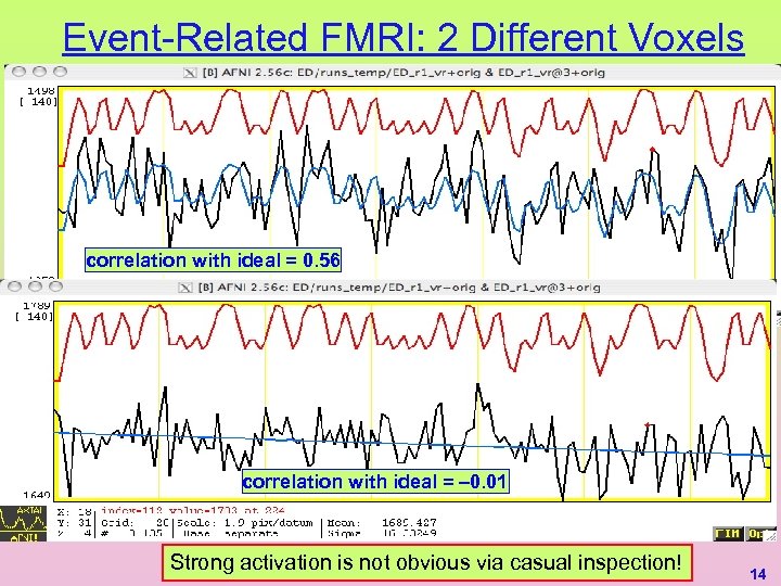
Event-Related FMRI: 2 Different Voxels correlation with ideal = 0. 56 correlation with ideal = – 0. 01 Strong activation is not obvious via casual inspection! 14
Time Series Analysis on Voxel Data • Most common forms of FMRI analysis • involve fitting the activation+BOLD model to each voxel’s time series separately (AKA “univariate” analysis) Result of model fits is a set of parameters at each voxel, estimated from that voxel’s data • e. g. , activation amplitude, delay, shape • “SPM” = statistical parametric map • Further analysis steps operate on individual SPMs • e. g. , combining/contrasting data among subjects 16
FMRI Activation Amplitude • Amplitude of activation (in one voxel, in one subject) = amplitude of model fitted to data • Usually fitted to all imaging runs simultaneously • Usually normalized to be in units of percent signal change from baseline (based on deoxy. HB theory) • Commonly have more than one category of stimulus/task • • e. g. , Image Viewing: Working Memory vs. Labeling Each category gets its own time series model All models fitted at once using multiple regression Each stimulus/task gets assigned its own amplitude 17
Multiple Stimuli = Multiple Regressors • Usually have more than one class of stimulus or activation in an experiment • e. g. , “face activation” vs “house activation” • Model each separate class of stimulus with a separate response function r 1(t ), r 2(t ), r 3(t ), … • Each rj (t ) is based on the stimulus timing for activity in class number j • Calculate j amplitude = amount of rj (t ) in voxel data time series Z(t ) • Contrast s to see which voxels have differential activation levels under different stimulus conditions • e. g. , statistical test on 1– 2 = 0 ? 18
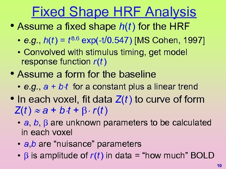
Fixed Shape HRF Analysis • Assume a fixed shape h(t ) for the HRF • e. g. , h(t ) = t 8. 6 exp(-t/0. 547) [MS Cohen, 1997] • Convolved with stimulus timing, get model response function r (t ) • Assume a form for the baseline • e. g. , a + b t for a constant plus a linear trend • In each voxel, fit data Z(t ) to curve of form Z(t ) a + b t + r (t ) • a, b, are unknown parameters to be calculated in each voxel • a, b are “nuisance” parameters • is amplitude of r (t ) in data = “how much” BOLD 19
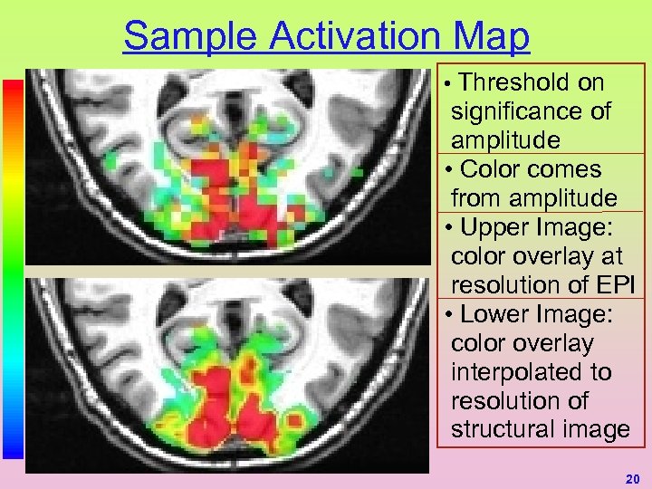
Sample Activation Map • Threshold on significance of amplitude • Color comes from amplitude • Upper Image: color overlay at resolution of EPI • Lower Image: color overlay interpolated to resolution of structural image 20
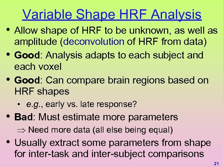
Variable Shape HRF Analysis • Allow shape of HRF to be unknown, as well as • • amplitude (deconvolution of HRF from data) Good: Analysis adapts to each subject and Good each voxel Good: Can compare brain regions based on Good HRF shapes • e. g. , early vs. late response? • Bad: Must estimate more parameters Bad Þ Need more data (all else being equal) • Usually extract some parameters from shape for inter-task and inter-subject comparisons 21
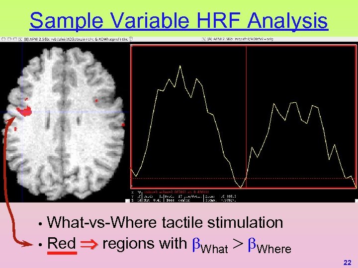
Sample Variable HRF Analysis Where HRF What-vs-Where tactile stimulation • Red regions with What Where • 22
Noise Issues in Time Series • Subject head movement • Biggest practical annoyance in FMRI • Physiological noise • Heartbeat and respiration affect signal in complex ways (e. g. , correlation in time and space) • Magnetic field fluctuations • Poorly understood and hard to correct: • Sometimes see 5 spikes in data with no apparent cause • Very slow signal drifts make long term experiments (e. g. , learning, adaptation) difficult 23
Inter-Subject Data Alignment • • Cortical folding patterns are (at least) as unique as fingerprints Inter-subject comparisons requires some way to bring brain regions into alignment • So that SPMs can be averaged and contrasted in various ways • Solutions: Brain Warping and ROIs 24
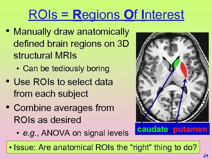
ROIs = Regions Of Interest • Manually draw anatomically defined brain regions on 3 D structural MRIs • Can be tediously boring • • Use ROIs to select data from each subject Combine averages from ROIs as desired • e. g. , ANOVA on signal levels caudate, putamen caudate • Issue: Are anatomical ROIs the “right” thing to do? 25
Easy Brain Warping • • Align brain volume so that inter-hemispheric fissure is vertical (z ), and Anterior-Posterior Commissure line is horizontal (y ) Stretch/shrink brain to fit Talairach-Tournoux Talairach Atlas dimensions Use (x, y, z) coordinates based at AC=(0, 0, 0) Accuracy: Not so good ( 5 -15 mm) Accuracy • FMRI analysts often spatially blur data or SPMs to adapt to this problem 26
Hard Brain Warping (3 D) • • • Nonlinearly distort (warp, morph, transform) brain volume images in 3 D to match sulcus-to -sulcus, gyrus-to-gyrus Very computationally intensive Accuracy: hard to gauge, since method is not Accuracy widely used • Good software for this is not readily available • Issue: Very large inter-subject variability even Issue in existence and shape of many sulci 27
Hard Brain Warping (2 D) • Idea: Warp brain only along cortical sheet Idea (triangulated 2 D surface model) rather than general 3 D transformation • Goal is still to align sulci and gyri (e. g. , by matching brain convexities) • Then create a new “standard” surface model, where nodes from all subjects are aligned • Does not deal with non-cortical structures • Hope: 2 D is a little easier than 3 D and may Hope • be more anatomically meaningful Not widely used at present • Software is available: Free. Surfer and Sure. Fit 28
Inter-Subject Analyses • • • Current methodologies are based on some sort of ANOVA (after alignment) • Alternative: PCA (etc) is not much used in FMRI Important to treat intra-subject and inter-subject variance separately • e. g. , paired and unpaired t-tests, and their generalizations in random-effects ANOVA • This point is not always appreciated Multi-way ANOVA is a method for structuring hypotheses and tests • Supplement with continuous covariates (e. g. , age)? • A proper analysis will need to be more general 29
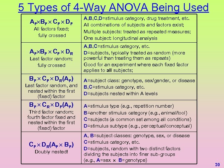
5 Types of 4 -Way ANOVA Being Used AF BF CF DF All factors fixed; fully crossed AF BF CF DR Last factor random; fully crossed BF CF DR(AF) Last factor random, and nested within the first (fixed) factor BF CR DF(AF) Third factor random; fourth factor fixed and nested within the first (fixed) factor CF DR(AF BF) Doubly nested! A, B, C, D=stimulus category, drug treatment, etc. All combinations of subjects and factors exist; Multiple subjects: treated as repeated measures; One subject: longitudinal analysis A, B, C=stimulus category, etc. D=subjects, typically treated as random (more powerful than treating them as repeats) Good for an experiment where each fixed factor applies to all subjects; A=subject class: genotype, sex/gender, or disease B, C=stimulus category, etc. D=subjects nested within A levels A=stimulus type (e. g. , repetition number) B=another stimulus category (e. g. , animal/tool) C=subjects (a common set among all conditions) D=stimulus subtype (e. g. , perceptual/conceptual) A, B=subject classes: genotype, sex, or disease C=stimulus category, etc. D=subjects, random with two distinct factors dividing the subjects into finer sub-groups (e. g. , A=sex B=genotype) 30
Standard FMRI Visualizations • • 2 D Grayscale anatomicals with functional activation percent change overlaid in color 3 orthgonal 2 D projections of activation maps • The SPM “glass brain” — very common in journal papers • • 3 D volume rendering 3 D rendering of cortical surface models • Analysis can also be performed directly on time series data projected to the cortical surface model — initial results are promising 31
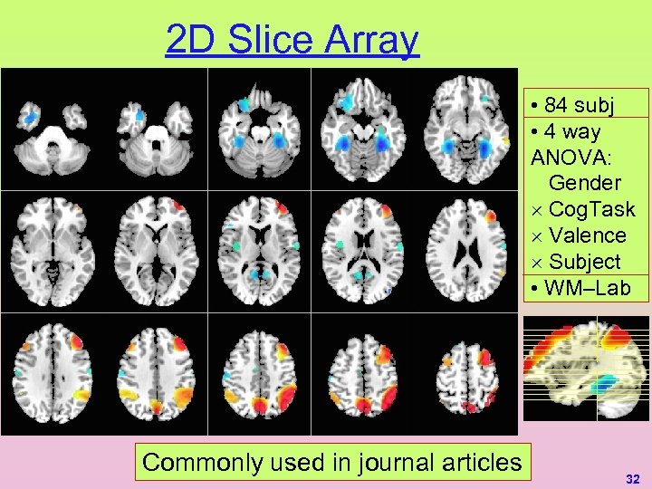
2 D Slice Array • 84 subj • 4 way ANOVA: Gender ´ Cog. Task ´ Valence ´ Subject • WM–Lab Commonly used in journal articles 32
3 D Volume Rendering • “Show Through” rendering: Color overlay above statistical threshold is projected outward to brain surface • 3 D structure becomes apparent from rotation of viewpoint 33
Cortical Surface Models • Color overlay above statistical threshold is intersected with surface model • Surface model can be inflated to see into sulci 34
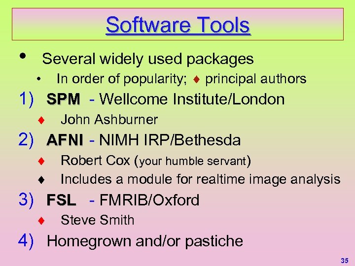
Software Tools • Several widely used packages • In order of popularity; principal authors 1) SPM - Wellcome Institute/London John Ashburner 2) AFNI - NIMH IRP/Bethesda Robert Cox (your humble servant) Includes a module for realtime image analysis 3) FSL - FMRIB/Oxford Steve Smith 4) Homegrown and/or pastiche 35
Points for Discussion & Comment • • Variations on standard FMRI time series analyses Directions in FMRI analysis research Things that are hard to do with FMRI Origins of fluctuations in FMRI activation amplitude • And what to do about them? • Visualization issues 36
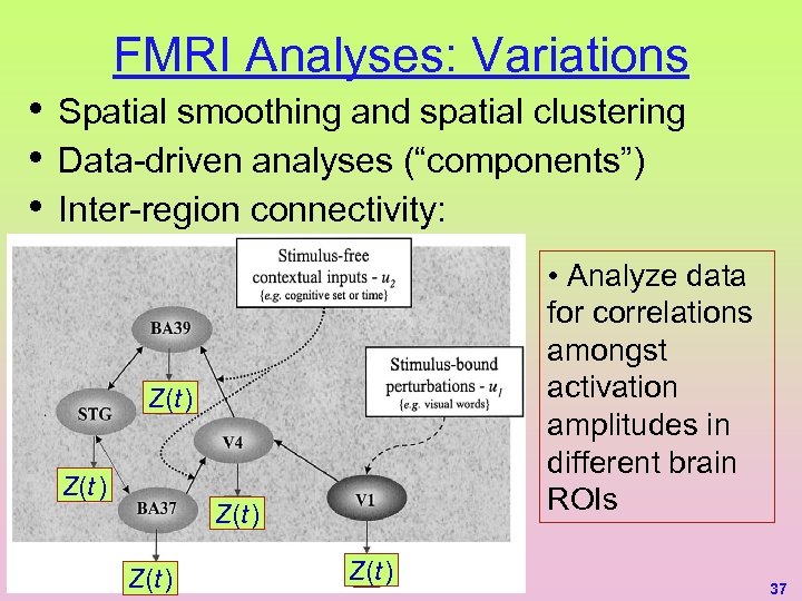
FMRI Analyses: Variations • • • Spatial smoothing and spatial clustering Data-driven analyses (“components”) Inter-region connectivity: • Analyze data for correlations amongst activation amplitudes in different brain ROIs Z(t ) Z(t ) 37
• FMRI Analysis Research Many “reasonable” space+time series analyses • Need methodologies for comparing them • • Combining data from multiple scanners/centers Closer integration of analysis to neural-level hypotheses f. MRI-DC • Cognitive models; signaling networks • Understand physiology better! • f. BIRN “Brainotyping”: methods for grouping and discriminating among brain maps • Application to individual patients? • Combining with X-omic data (X=gene, protein, …)? 38
Some Things That Are Hard in FMRI • Measuring neural effects that take a long time to occur (ten minutes or more) • • • Learning, adaptation; Effects of some drugs Measuring neural effects associated with tasks that require big subject movements • Continuous speech; swallowing; head movement Distinguishing neural events closer than ~500 ms in time Measuring activation in brainstem nuclei Measuring differences in timing or strength of neural activity between brain regions Characterizing individual subject phenotypes 39
FMRI Amplitude Fluctuations • • Task type (often the principal concern) Subject type (concern? or confound? or both? ) • Disease status, genotype, sex, age, … Subject task performance (behavior, attention) Neural “activation” level (whatever that is) Physiological noise (heartbeat, breathing) Task-related noise • Movement artifacts, breathing changes, … Subject’s hemo-response • Different shapes, OEFs, vasculature, … Subject monitoring and calibration? 40
Issues in Visualization • Regions below statistical threshold: • translucency? topographically? animation? • • • Multi-subject data - beyond averages? Connectivity maps - inter-regional correlations? Dynamic Causal Modeling? High dimensional patterns that activate much of the brain • e. g. , Watching a movie • Basic problem: even after filtering out much problem of the crap, are left with high-dimensional info at each place in a 3 D space 42
Finally … Thanks • The list of people I should thank is not quite endless … MM Klosek. JS Hyde. JR Binder. EA De. Yoe. SM Rao. EA Stein. A Jesmanowicz. MS Beauchamp. BD Ward. KM Donahue. PA Bandettini. AS Bloom. T Ross. M Huerta. ZS Saad. K Ropella. B Knutson. J Bobholz. G Chen. RM Birn. J Ratke. PSF Bellgowan. J Frost. K Bove-Bettis. R Doucette. RC Reynolds. PP Christidis. LR Frank. R Desimone. L Ungerleider. KR Hammett. A Clark. DS Cohen. DA Jacobson. JA Sidles. EC Wong. Et alii … 43
6e88486075749c3693f797db2e3e2c2a.ppt