3a51e6eb3073412be00eb586a86ec92c.ppt
- Количество слайдов: 85
+ Probability & Random Variables
+ Probability & Random Variables n Randomness, n Probability Rules n Conditional n Probability, and Simulation Probability and Independence Discrete and Continuous Random Variables n Transforming n Binomial and Combining Random Variables and Geometric Random Variables
+ Randomness, Probability, and Simulation Learning Objectives After this section, you should be able to… ü DESCRIBE the idea of probability ü DESCRIBE myths about randomness ü DESIGN and PERFORM simulations
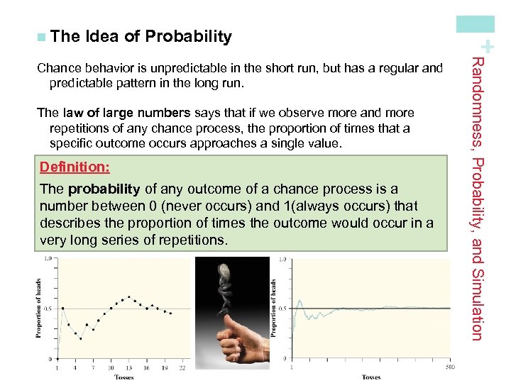
Idea of Probability The law of large numbers says that if we observe more and more repetitions of any chance process, the proportion of times that a specific outcome occurs approaches a single value. Definition: The probability of any outcome of a chance process is a number between 0 (never occurs) and 1(always occurs) that describes the proportion of times the outcome would occur in a very long series of repetitions. Randomness, Probability, and Simulation Chance behavior is unpredictable in the short run, but has a regular and predictable pattern in the long run. + n The
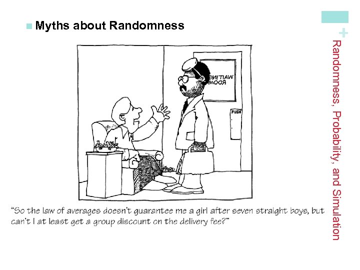
about Randomness The myth of short-run regularity: The idea of probability is that randomness is predictable in the long run. Our intuition tries to tell us random phenomena should also be predictable in the short run. However, probability does not allow us to make short-run predictions. The myth of the “law of averages”: Probability tells us random behavior evens out in the long run. Future outcomes are not affected by past behavior. That is, past outcomes do not influence the likelihood of individual outcomes occurring in the future. Randomness, Probability, and Simulation The idea of probability seems straightforward. However, there are several myths of chance behavior we must address. + n Myths
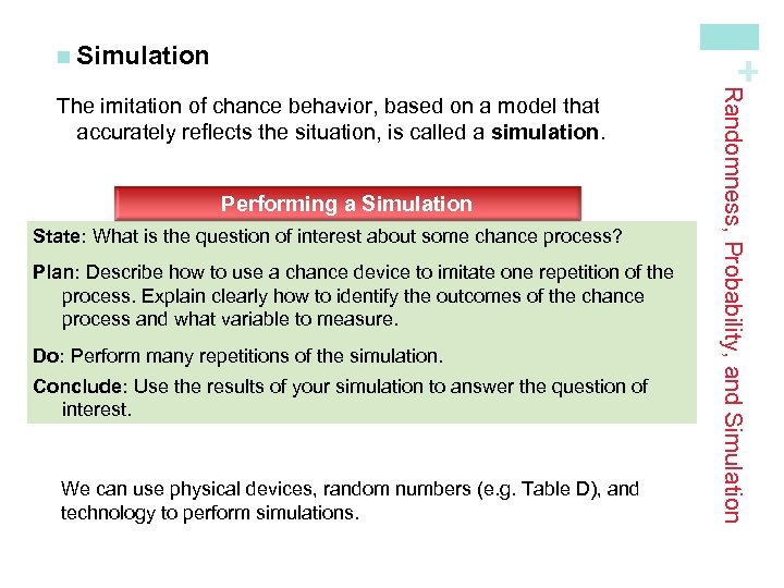
+ n Simulation Performing a Simulation State: What is the question of interest about some chance process? Plan: Describe how to use a chance device to imitate one repetition of the process. Explain clearly how to identify the outcomes of the chance process and what variable to measure. Do: Perform many repetitions of the simulation. Conclude: Use the results of your simulation to answer the question of interest. We can use physical devices, random numbers (e. g. Table D), and technology to perform simulations. Randomness, Probability, and Simulation The imitation of chance behavior, based on a model that accurately reflects the situation, is called a simulation.
+ Golden Ticket Lottery n Golden Ticket Parking Lottery n At a local high school, 95 students have permission to park on campus. Each month, the student council holds a “golden ticket parking lottery” at a school assembly. The two lucky winners are given reserved parking spots next to the school’s main entrance. Last month, the winning tickets were drawn by a student council member from the AP Statistics class. When both golden tickets went to members of that same class, some people thought the lottery had been rigged. There are 28 students in the AP Statistics class, all of whom are eligible to park on campus. Design and carry out a simulation to decide whether it’s plausible that the lottery was carried out fairly.
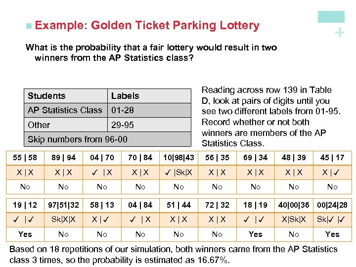
Golden Ticket Parking Lottery + n Example: What is the probability that a fair lottery would result in two winners from the AP Statistics class? Students Reading across row 139 in Table D, look at pairs of digits until you see two different labels from 01 -95. Record whether or not both winners are members of the AP Statistics Class. Labels AP Statistics Class 01 -28 Other 29 -95 Skip numbers from 96 -00 55 | 58 89 | 94 04 | 70 70 | 84 10|98|43 56 | 35 69 | 34 48 | 39 45 | 17 X|X ✓ |X X|X ✓ |Sk|X X|X X|✓ No No No 19 | 12 97|51|32 58 | 13 04 | 84 51 | 44 72 | 32 18 | 19 ✓ |✓ Sk|X|X X|✓ ✓ |X X|X ✓ |✓ X|Sk|X Sk|✓ |✓ Yes No No No Yes 40|00|36 00|24|28 Based on 18 repetitions of our simulation, both winners came from the AP Statistics class 3 times, so the probability is estimated as 16. 67%.
+ NASCAR Cards & Cereal Boxes n Simulations with technology n In an attempt to increase sales, a breakfast cereal company decides to offer a NASCAR promotion. Each box of cereal will contain a collectible card featuring one of these NASCAR drivers: Jeff Gordon, Dale Earnhardt, Jr. , Tony Stewart, Danica Patrick, or Jimmie Johnson. The company says that each of the 5 cards is equally likely to appear in any box of cereal. A NASCAR fan decides to keep buying boxes of the cereal until she has all 5 drivers’ cards. She is surprised when it takes her 23 boxes to get the full set of cards. Should she be surprised? Design and carry out a simulation to help answer this question.
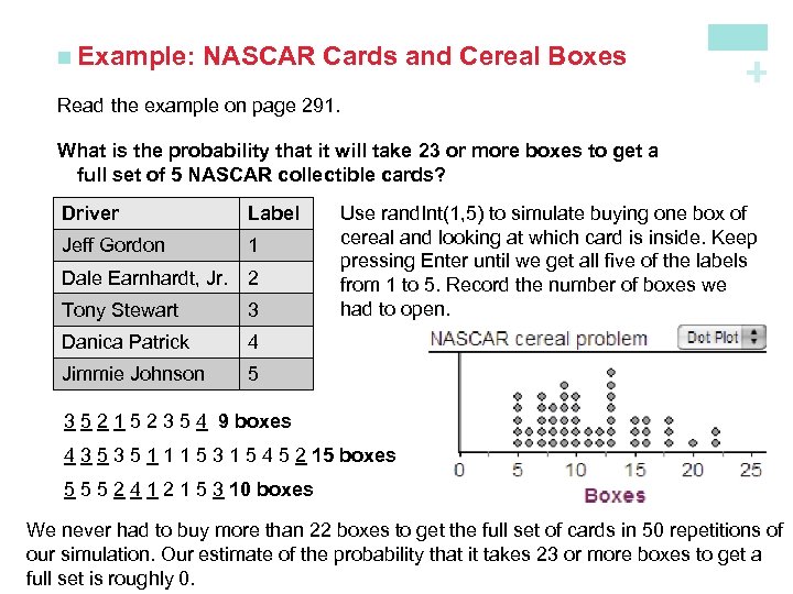
NASCAR Cards and Cereal Boxes + n Example: Read the example on page 291. What is the probability that it will take 23 or more boxes to get a full set of 5 NASCAR collectible cards? Driver Label Jeff Gordon 1 Dale Earnhardt, Jr. 2 Tony Stewart 3 Danica Patrick 4 Jimmie Johnson Use rand. Int(1, 5) to simulate buying one box of cereal and looking at which card is inside. Keep pressing Enter until we get all five of the labels from 1 to 5. Record the number of boxes we had to open. 5 3 5 2 1 5 2 3 5 4 9 boxes 4 3 5 1 1 1 5 3 1 5 4 5 2 15 boxes 5 5 5 2 4 1 2 1 5 3 10 boxes We never had to buy more than 22 boxes to get the full set of cards in 50 repetitions of our simulation. Our estimate of the probability that it takes 23 or more boxes to get a full set is roughly 0.
+ Probability Rules Learning Objectives After this section, you should be able to… ü DESCRIBE chance behavior with a probability model ü DEFINE and APPLY basic rules of probability ü DETERMINE probabilities from two-way tables ü CONSTRUCT Venn diagrams and DETERMINE probabilities
Models Descriptions of chance behavior contain two parts: Definition: The sample space S of a chance process is the set of all possible outcomes. A probability model is a description of some chance process that consists of two parts: a sample space S and a probability for each outcome. Probability Rules In Section 5. 1, we used simulation to imitate chance behavior. Fortunately, we don’t have to always rely on simulations to determine the probability of a particular outcome. + n Probability
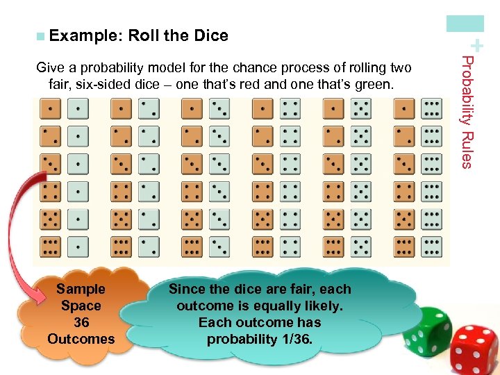
Roll the Dice Sample Space 36 Outcomes Since the dice are fair, each outcome is equally likely. Each outcome has probability 1/36. Probability Rules Give a probability model for the chance process of rolling two fair, six-sided dice – one that’s red and one that’s green. + n Example:
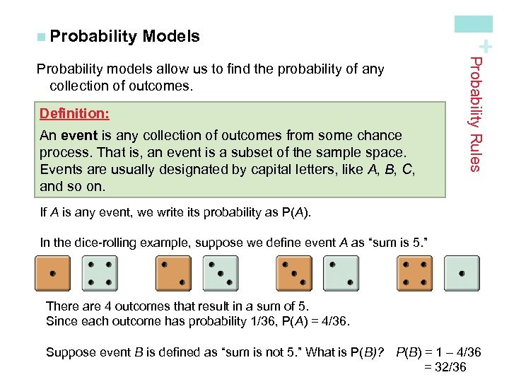
Models Definition: An event is any collection of outcomes from some chance process. That is, an event is a subset of the sample space. Events are usually designated by capital letters, like A, B, C, and so on. Probability Rules Probability models allow us to find the probability of any collection of outcomes. + n Probability If A is any event, we write its probability as P(A). In the dice-rolling example, suppose we define event A as “sum is 5. ” There are 4 outcomes that result in a sum of 5. Since each outcome has probability 1/36, P(A) = 4/36. Suppose event B is defined as “sum is not 5. ” What is P(B)? P(B) = 1 – 4/36 = 32/36
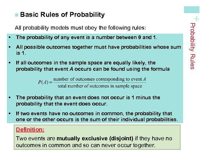
Rules of Probability § The probability of any event is a number between 0 and 1. § All possible outcomes together must have probabilities whose sum is 1. § If all outcomes in the sample space are equally likely, the probability that event A occurs can be found using the formula § The probability that an event does not occur is 1 minus the probability that the event does occur. § If two events have no outcomes in common, the probability that one or the other occurs is the sum of their individual probabilities. Definition: Two events are mutually exclusive (disjoint) if they have no outcomes in common and so can never occur together. Probability Rules All probability models must obey the following rules: + n Basic
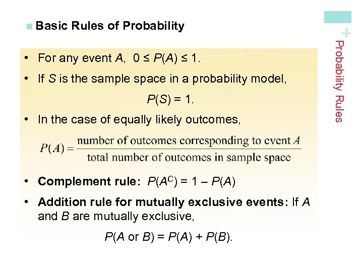
Rules of Probability • If S is the sample space in a probability model, P(S) = 1. • In the case of equally likely outcomes, • Complement rule: P(AC) = 1 – P(A) • Addition rule for mutually exclusive events: If A and B are mutually exclusive, P(A or B) = P(A) + P(B). Probability Rules • For any event A, 0 ≤ P(A) ≤ 1. + n Basic
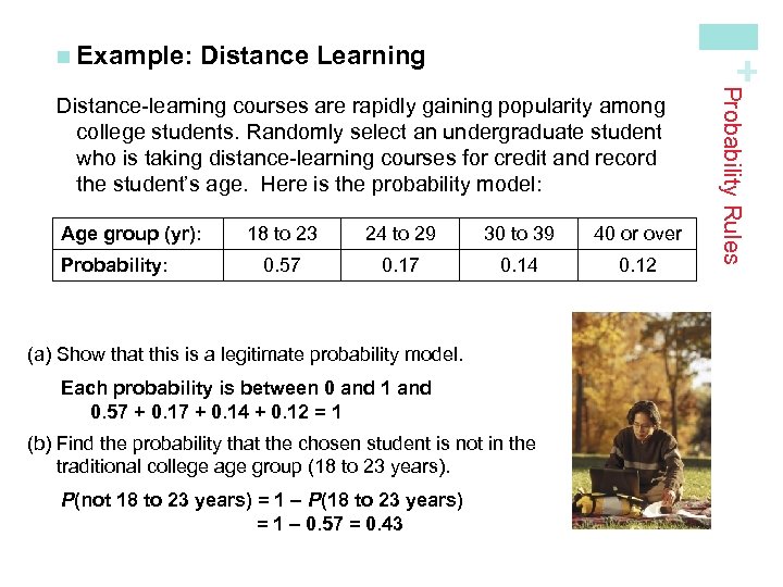
Distance Learning + n Example: Age group (yr): Probability: 18 to 23 24 to 29 30 to 39 40 or over 0. 57 0. 14 0. 12 (a) Show that this is a legitimate probability model. Each probability is between 0 and 1 and 0. 57 + 0. 14 + 0. 12 = 1 (b) Find the probability that the chosen student is not in the traditional college age group (18 to 23 years). P(not 18 to 23 years) = 1 – P(18 to 23 years) = 1 – 0. 57 = 0. 43 Probability Rules Distance-learning courses are rapidly gaining popularity among college students. Randomly select an undergraduate student who is taking distance-learning courses for credit and record the student’s age. Here is the probability model:
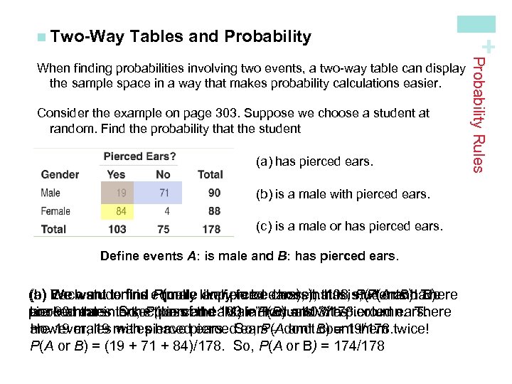
Tables and Probability Consider the example on page 303. Suppose we choose a student at random. Find the probability that the student (a) has pierced ears. (b) is a male with pierced ears. (c) is a male or has pierced ears. Define events A: is male and B: has pierced ears. (a) Each student is equally likelypierced ears), that is, P(A and There (c) (b) We want to find P(male or pierced ears), that is, students have and to be chosen. 103 P(A or B). piercedmales in the class and 103 = P(B) = 103/178. column. There are 90 the intersection of the “Male” row and “Yes” Look at ears. So, P(pierced ears) individuals with pierced ears. However, 19 with pierced ears – and count them are 19 males have pierced. So, P(Adon’t B) = 19/178. twice! P(A or B) = (19 + 71 + 84)/178. So, P(A or B) = 174/178 Probability Rules When finding probabilities involving two events, a two-way table can display the sample space in a way that makes probability calculations easier. + n Two-Way
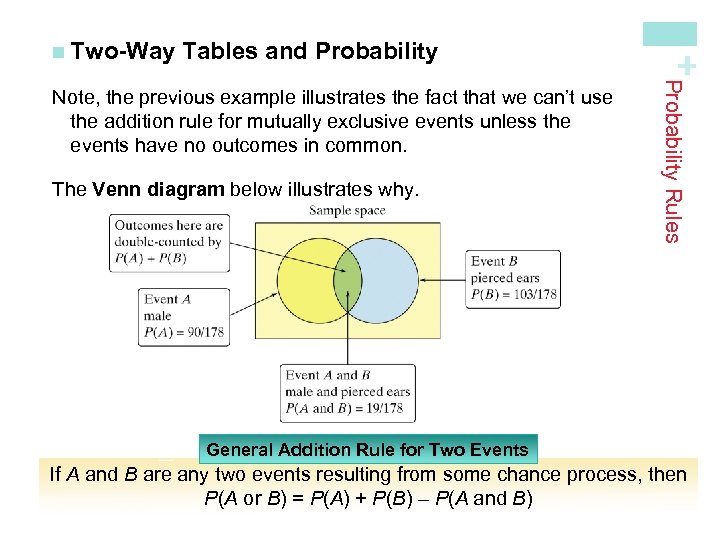
Tables and Probability The Venn diagram below illustrates why. Probability Rules Note, the previous example illustrates the fact that we can’t use the addition rule for mutually exclusive events unless the events have no outcomes in common. + n Two-Way General Addition Rule for Two Events If A and B are any two events resulting from some chance process, then P(A or B) = P(A) + P(B) – P(A and B)
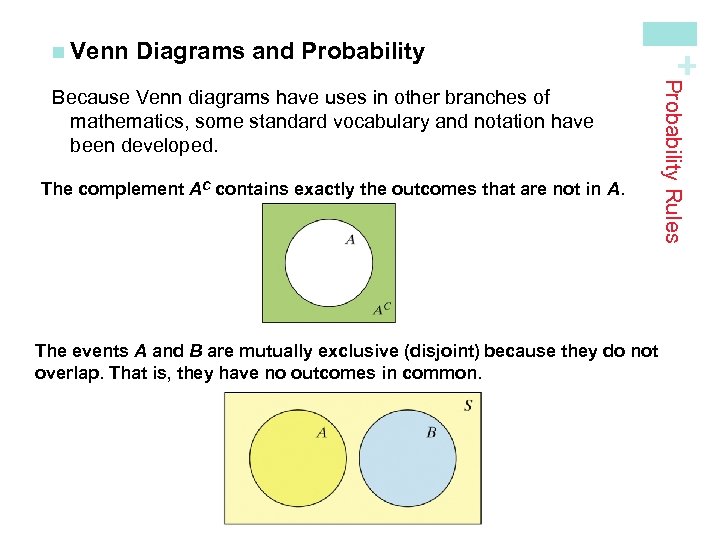
Diagrams and Probability The complement AC contains exactly the outcomes that are not in A. The events A and B are mutually exclusive (disjoint) because they do not overlap. That is, they have no outcomes in common. Probability Rules Because Venn diagrams have uses in other branches of mathematics, some standard vocabulary and notation have been developed. + n Venn
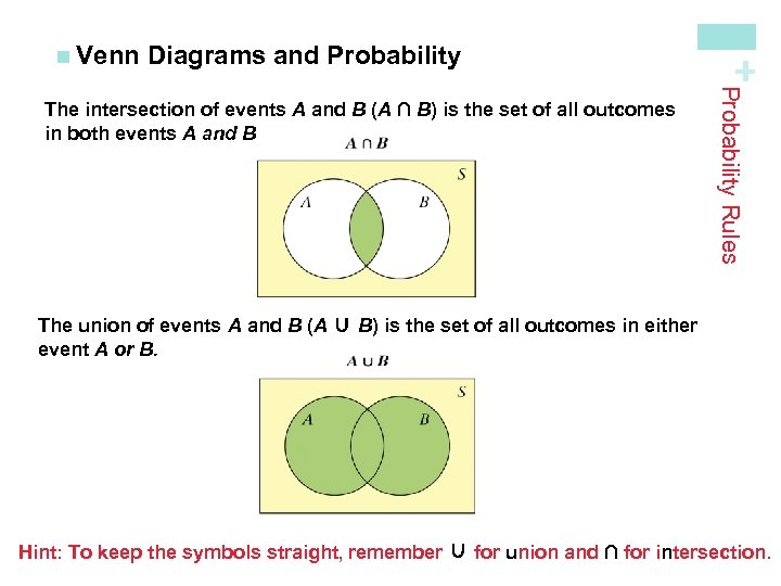
Diagrams and Probability Rules The intersection of events A and B (A ∩ B) is the set of all outcomes in both events A and B. + n Venn The union of events A and B (A ∪ B) is the set of all outcomes in either event A or B. Hint: To keep the symbols straight, remember ∪ for union and ∩ for intersection.
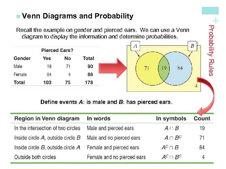
Diagrams and Probability Define events A: is male and B: has pierced ears. Probability Rules Recall the example on gender and pierced ears. We can use a Venn diagram to display the information and determine probabilities. + n Venn
+Conditional Probability and Independence Learning Objectives After this section, you should be able to… ü DEFINE conditional probability ü COMPUTE conditional probabilities ü DESCRIBE chance behavior with a tree diagram ü DEFINE independent events ü DETERMINE whether two events are independent ü APPLY the general multiplication rule to solve probability questions
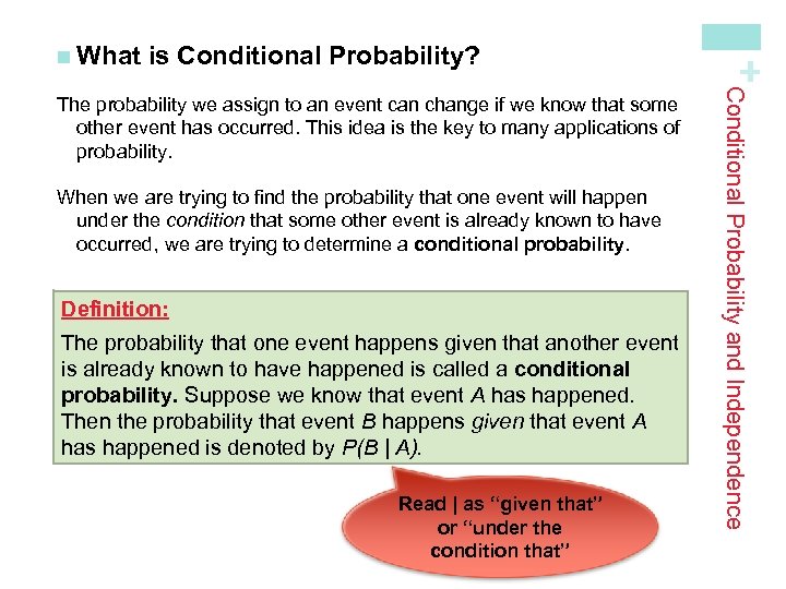
is Conditional Probability? When we are trying to find the probability that one event will happen under the condition that some other event is already known to have occurred, we are trying to determine a conditional probability. Definition: The probability that one event happens given that another event is already known to have happened is called a conditional probability. Suppose we know that event A has happened. Then the probability that event B happens given that event A has happened is denoted by P(B | A). Read | as “given that” or “under the condition that” Conditional Probability and Independence The probability we assign to an event can change if we know that some other event has occurred. This idea is the key to many applications of probability. + n What
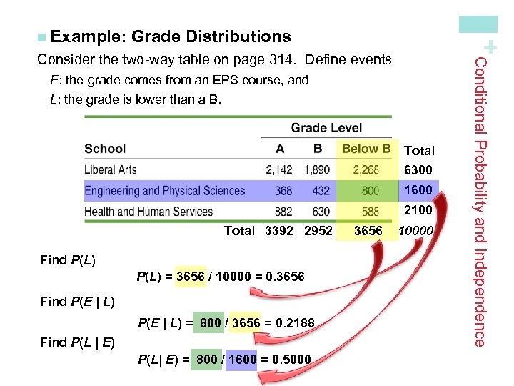
Grade Distributions + n Example: E: the grade comes from an EPS course, and L: the grade is lower than a B. Total 6300 1600 2100 Total 3392 2952 Find P(L) = 3656 / 10000 = 0. 3656 Find P(E | L) = 800 / 3656 = 0. 2188 Find P(L | E) P(L| E) = 800 / 1600 = 0. 5000 3656 10000 Conditional Probability and Independence Consider the two-way table on page 314. Define events
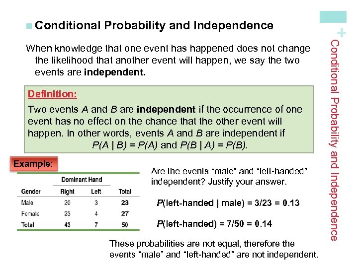
Probability and Independence Definition: Two events A and B are independent if the occurrence of one event has no effect on the chance that the other event will happen. In other words, events A and B are independent if P(A | B) = P(A) and P(B | A) = P(B). Example: Are the events “male” and “left-handed” independent? Justify your answer. P(left-handed | male) = 3/23 = 0. 13 P(left-handed) = 7/50 = 0. 14 These probabilities are not equal, therefore the events “male” and “left-handed” are not independent. Conditional Probability and Independence When knowledge that one event has happened does not change the likelihood that another event will happen, we say the two events are independent. + n Conditional
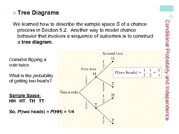
Diagrams Consider flipping a coin twice. What is the probability of getting two heads? Sample Space: HH HT TH TT So, P(two heads) = P(HH) = 1/4 Conditional Probability and Independence We learned how to describe the sample space S of a chance process in Section 5. 2. Another way to model chance behavior that involves a sequence of outcomes is to construct a tree diagram. + n Tree
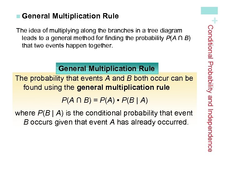
Multiplication Rule General Multiplication Rule The probability that events A and B both occur can be found using the general multiplication rule P(A ∩ B) = P(A) • P(B | A) where P(B | A) is the conditional probability that event B occurs given that event A has already occurred. Conditional Probability and Independence The idea of multiplying along the branches in a tree diagram leads to a general method for finding the probability P(A ∩ B) that two events happen together. + n General
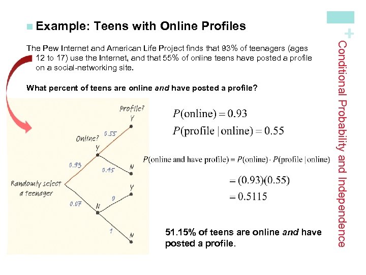
Teens with Online Profiles What percent of teens are online and have posted a profile? 51. 15% of teens are online and have posted a profile. Conditional Probability and Independence The Pew Internet and American Life Project finds that 93% of teenagers (ages 12 to 17) use the Internet, and that 55% of online teens have posted a profile on a social-networking site. + n Example:
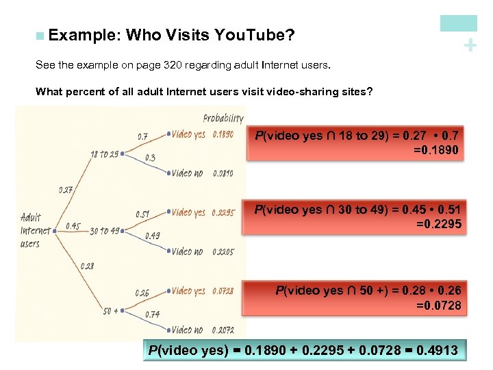
Who Visits You. Tube? + n Example: See the example on page 320 regarding adult Internet users. What percent of all adult Internet users visit video-sharing sites? P(video yes ∩ 18 to 29) = 0. 27 • 0. 7 =0. 1890 P(video yes ∩ 30 to 49) = 0. 45 • 0. 51 =0. 2295 P(video yes ∩ 50 +) = 0. 28 • 0. 26 =0. 0728 P(video yes) = 0. 1890 + 0. 2295 + 0. 0728 = 0. 4913
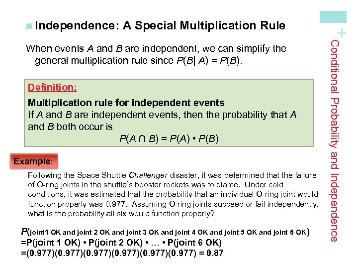
A Special Multiplication Rule Definition: Multiplication rule for independent events If A and B are independent events, then the probability that A and B both occur is P(A ∩ B) = P(A) • P(B) Example: Following the Space Shuttle Challenger disaster, it was determined that the failure of O-ring joints in the shuttle’s booster rockets was to blame. Under cold conditions, it was estimated that the probability that an individual O-ring joint would function properly was 0. 977. Assuming O-ring joints succeed or fail independently, what is the probability all six would function properly? P(joint 1 OK and joint 2 OK and joint 3 OK and joint 4 OK and joint 5 OK and joint 6 OK ) =P(joint 1 OK) • P(joint 2 OK) • … • P(joint 6 OK) =(0. 977)(0. 977) = 0. 87 Conditional Probability and Independence When events A and B are independent, we can simplify the general multiplication rule since P(B| A) = P(B). + n Independence:
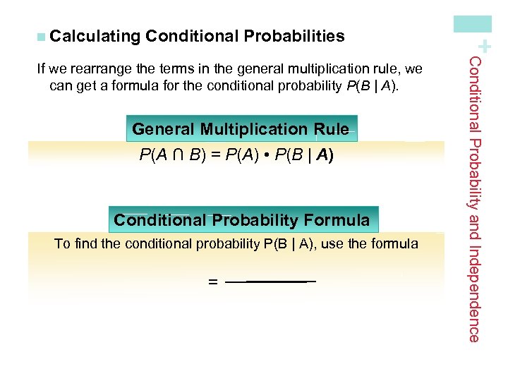
Conditional Probabilities General Multiplication Rule P(A ∩ B) = P(A) • P(B | A) Conditional Probability Formula To find the conditional probability P(B | A), use the formula = Conditional Probability and Independence If we rearrange the terms in the general multiplication rule, we can get a formula for the conditional probability P(B | A). + n Calculating
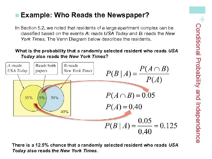
Who Reads the Newspaper? What is the probability that a randomly selected resident who reads USA Today also reads the New York Times? There is a 12. 5% chance that a randomly selected resident who reads USA Today also reads the New York Times. Conditional Probability and Independence In Section 5. 2, we noted that residents of a large apartment complex can be classified based on the events A: reads USA Today and B: reads the New York Times. The Venn Diagram below describes the residents. + n Example:
+ Discrete and Continuous Random Variables Learning Objectives After this section, you should be able to… ü APPLY the concept of discrete random variables to a variety of statistical settings ü CALCULATE and INTERPRET the mean (expected value) of a discrete random variable ü CALCULATE and INTERPRET the standard deviation (and variance) of a discrete random variable ü DESCRIBE continuous random variables
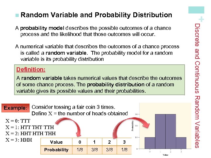
Variable and Probability Distribution A numerical variable that describes the outcomes of a chance process is called a random variable. The probability model for a random variable is its probability distribution Definition: A random variable takes numerical values that describe the outcomes of some chance process. The probability distribution of a random variable gives its possible values and their probabilities. Example: Consider tossing a fair coin 3 times. Define X = the number of heads obtained X = 0: TTT X = 1: HTT THT TTH X = 2: HHT HTH THH X = 3: HHH Value 0 1 2 3 Probability 1/8 3/8 1/8 Discrete and Continuous Random Variables A probability model describes the possible outcomes of a chance process and the likelihood that those outcomes will occur. + n Random
Random Variables + n Discrete Random Variables and Their Probability Distributions A discrete random variable X takes a fixed set of possible values with gaps between. The probability distribution of a discrete random variable X lists the values xi and their probabilities pi: Value: x 1 Probability: p 1 x 2 p 2 x 3 p 3 … … The probabilities pi must satisfy two requirements: 1. Every probability pi is a number between 0 and 1. 2. The sum of the probabilities is 1. To find the probability of any event, add the probabilities pi of the particular values xi that make up the event. Discrete and Continuous Random Variables There are two main types of random variables: discrete and continuous. If we can find a way to list all possible outcomes for a random variable and assign probabilities to each one, we have a discrete random variable.
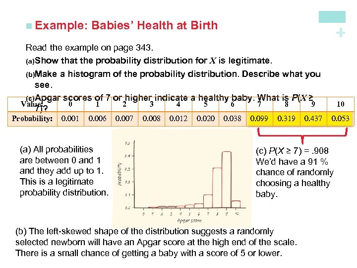
Babies’ Health at Birth + n Example: Read the example on page 343. (a) Show that the probability distribution for X is legitimate. (b)Make a histogram of the probability distribution. Describe what you see. (c) Apgar scores of 7 or higher indicate a healthy baby. What is P(X ≥ Value: 0 1 2 3 4 5 6 7 8 9 7)? Probability: 0. 001 0. 006 (a) All probabilities are between 0 and 1 and they add up to 1. This is a legitimate probability distribution. 0. 007 0. 008 0. 012 0. 020 0. 038 0. 099 0. 319 0. 437 10 0. 053 (c) P(X ≥ 7) =. 908 We’d have a 91 % chance of randomly choosing a healthy baby. (b) The left-skewed shape of the distribution suggests a randomly selected newborn will have an Apgar score at the high end of the scale. There is a small chance of getting a baby with a score of 5 or lower.
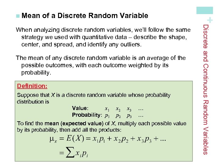
of a Discrete Random Variable The mean of any discrete random variable is an average of the possible outcomes, with each outcome weighted by its probability. Definition: Suppose that X is a discrete random variable whose probability distribution is Value: x 1 x 2 x 3 … Probability: p 1 p 2 p 3 … To find the mean (expected value) of X, multiply each possible value by its probability, then add all the products: Discrete and Continuous Random Variables When analyzing discrete random variables, we’ll follow the same strategy we used with quantitative data – describe the shape, center, and spread, and identify any outliers. + n Mean
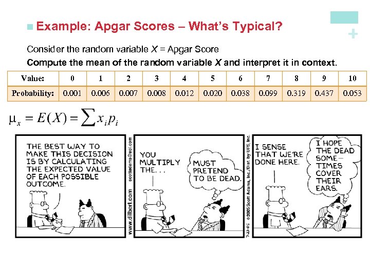
Apgar Scores – What’s Typical? + n Example: Consider the random variable X = Apgar Score Compute the mean of the random variable X and interpret it in context. Value: 0 1 2 3 4 5 6 7 8 9 10 Probability: 0. 001 0. 006 0. 007 0. 008 0. 012 0. 020 0. 038 0. 099 0. 319 0. 437 0. 053 The mean Apgar score of a randomly selected newborn is 8. 128. This is the longterm average Agar score of many, many randomly chosen babies. Note: The expected value does not need to be a possible value of X or an integer! It is a long-term average over many repetitions.
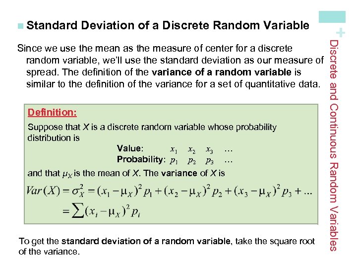
Deviation of a Discrete Random Variable Definition: Suppose that X is a discrete random variable whose probability distribution is Value: x 1 x 2 x 3 … Probability: p 1 p 2 p 3 … and that µX is the mean of X. The variance of X is To get the standard deviation of a random variable, take the square root of the variance. Discrete and Continuous Random Variables Since we use the mean as the measure of center for a discrete random variable, we’ll use the standard deviation as our measure of spread. The definition of the variance of a random variable is similar to the definition of the variance for a set of quantitative data. + n Standard
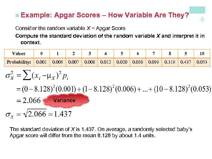
Apgar Scores – How Variable Are They? + n Example: Consider the random variable X = Apgar Score Compute the standard deviation of the random variable X and interpret it in context. Value: 0 1 2 3 4 5 6 7 8 9 10 Probability: 0. 001 0. 006 0. 007 0. 008 0. 012 0. 020 0. 038 0. 099 0. 319 0. 437 0. 053 Variance The standard deviation of X is 1. 437. On average, a randomly selected baby’s Apgar score will differ from the mean 8. 128 by about 1. 4 units.
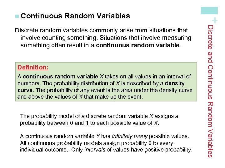
Random Variables Definition: A continuous random variable X takes on all values in an interval of numbers. The probability distribution of X is described by a density curve. The probability of any event is the area under the density curve and above the values of X that make up the event. The probability model of a discrete random variable X assigns a probability between 0 and 1 to each possible value of X. A continuous random variable Y has infinitely many possible values. All continuous probability models assign probability 0 to every individual outcome. Only intervals of values have positive probability. Discrete and Continuous Random Variables Discrete random variables commonly arise from situations that involve counting something. Situations that involve measuring something often result in a continuous random variable. + n Continuous
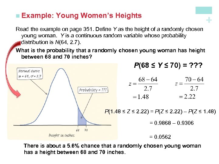
Young Women’s Heights + n Example: Read the example on page 351. Define Y as the height of a randomly chosen young woman. Y is a continuous random variable whose probability distribution is N(64, 2. 7). What is the probability that a randomly chosen young woman has height between 68 and 70 inches? P(68 ≤ Y ≤ 70) = ? ? ? P(1. 48 ≤ Z ≤ 2. 22) = P(Z ≤ 2. 22) – P(Z ≤ 1. 48) = 0. 9868 – 0. 9306 = 0. 0562 There is about a 5. 6% chance that a randomly chosen young woman has a height between 68 and 70 inches.
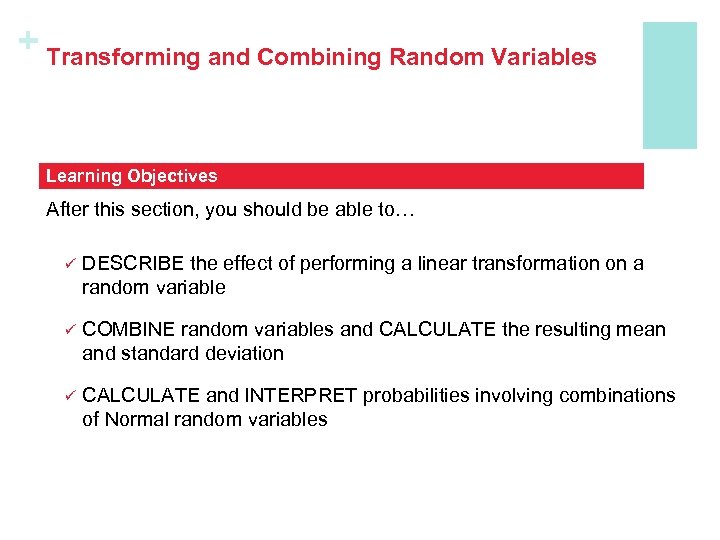
+ Transforming and Combining Random Variables Learning Objectives After this section, you should be able to… ü DESCRIBE the effect of performing a linear transformation on a random variable ü COMBINE random variables and CALCULATE the resulting mean and standard deviation ü CALCULATE and INTERPRET probabilities involving combinations of Normal random variables
Transformations In Chapter 2, we studied the effects of linear transformations on the shape, center, and spread of a distribution of data. Recall: 1. Adding (or subtracting) a constant, a, to each observation: • Adds a to measures of center and location. • Does not change the shape or measures of spread. 2. Multiplying (or dividing) each observation by a constant, b: • Multiplies (divides) measures of center and location by b. • Multiplies (divides) measures of spread by |b|. • Does not change the shape of the distribution. Transforming and Combining Random Variables In Section 6. 1, we learned that the mean and standard deviation give us important information about a random variable. In this section, we’ll learn how the mean and standard deviation are affected by transformations on random variables. + n Linear
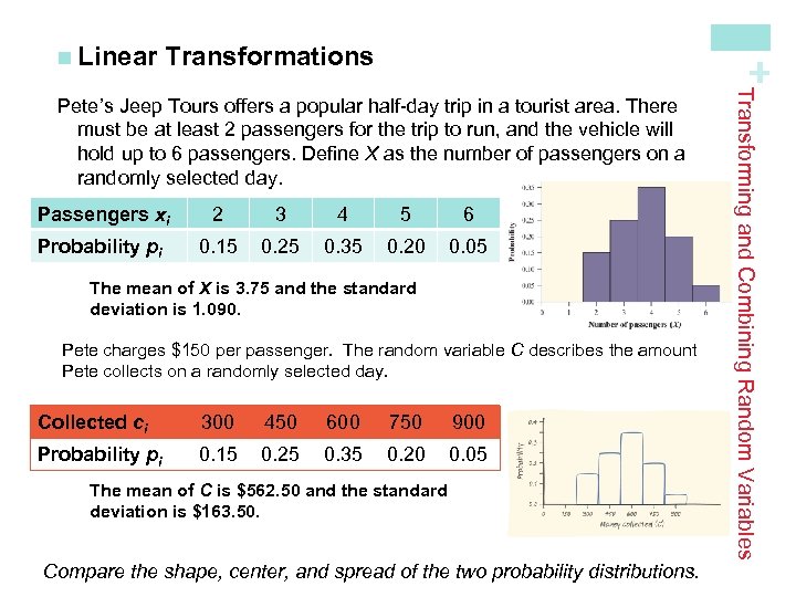
Transformations + n Linear Passengers xi 2 3 4 5 6 Probability pi 0. 15 0. 25 0. 35 0. 20 0. 05 The mean of X is 3. 75 and the standard deviation is 1. 090. Pete charges $150 per passenger. The random variable C describes the amount Pete collects on a randomly selected day. Collected ci 300 450 600 750 900 Probability pi 0. 15 0. 25 0. 35 0. 20 0. 05 The mean of C is $562. 50 and the standard deviation is $163. 50. Compare the shape, center, and spread of the two probability distributions. Transforming and Combining Random Variables Pete’s Jeep Tours offers a popular half-day trip in a tourist area. There must be at least 2 passengers for the trip to run, and the vehicle will hold up to 6 passengers. Define X as the number of passengers on a randomly selected day.
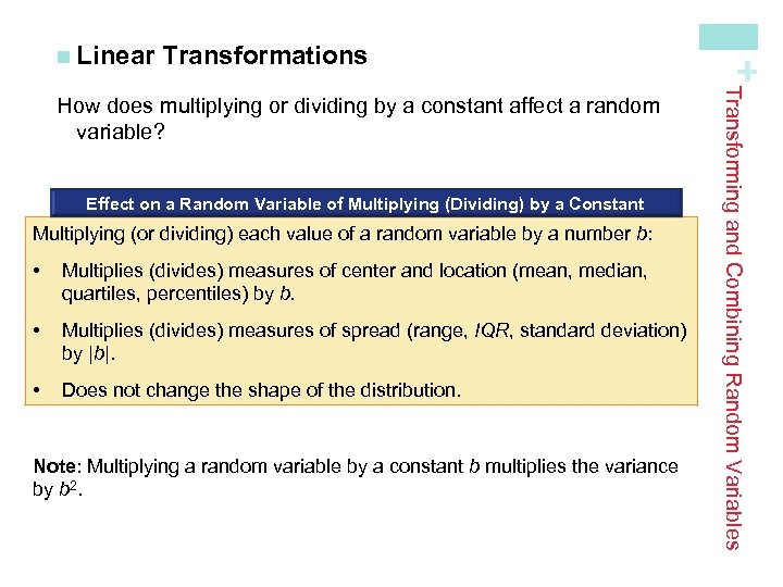
Transformations Effect on a Random Variable of Multiplying (Dividing) by a Constant Multiplying (or dividing) each value of a random variable by a number b: • Multiplies (divides) measures of center and location (mean, median, quartiles, percentiles) by b. • Multiplies (divides) measures of spread (range, IQR, standard deviation) by |b|. • Does not change the shape of the distribution. Note: Multiplying a random variable by a constant b multiplies the variance by b 2. Transforming and Combining Random Variables How does multiplying or dividing by a constant affect a random variable? + n Linear
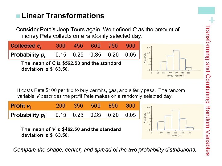
Transformations + n Linear Collected ci 300 450 600 750 900 Probability pi 0. 15 0. 25 0. 35 0. 20 0. 05 The mean of C is $562. 50 and the standard deviation is $163. 50. It costs Pete $100 per trip to buy permits, gas, and a ferry pass. The random variable V describes the profit Pete makes on a randomly selected day. Profit vi 200 350 500 650 800 Probability pi 0. 15 0. 25 0. 35 0. 20 0. 05 The mean of V is $462. 50 and the standard deviation is $163. 50. Compare the shape, center, and spread of the two probability distributions. Transforming and Combining Random Variables Consider Pete’s Jeep Tours again. We defined C as the amount of money Pete collects on a randomly selected day.
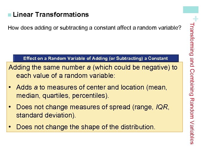
Transformations Effect on a Random Variable of Adding (or Subtracting) a Constant Adding the same number a (which could be negative) to each value of a random variable: • Adds a to measures of center and location (mean, median, quartiles, percentiles). • Does not change measures of spread (range, IQR, standard deviation). • Does not change the shape of the distribution. Transforming and Combining Random Variables How does adding or subtracting a constant affect a random variable? + n Linear
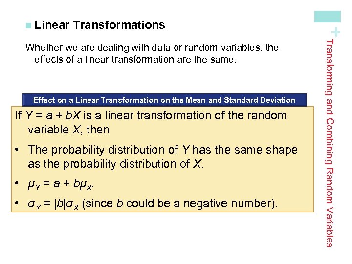
Transformations Effect on a Linear Transformation on the Mean and Standard Deviation If Y = a + b. X is a linear transformation of the random variable X, then • The probability distribution of Y has the same shape as the probability distribution of X. • µY = a + bµX. • σY = |b|σX (since b could be a negative number). Transforming and Combining Random Variables Whether we are dealing with data or random variables, the effects of a linear transformation are the same. + n Linear
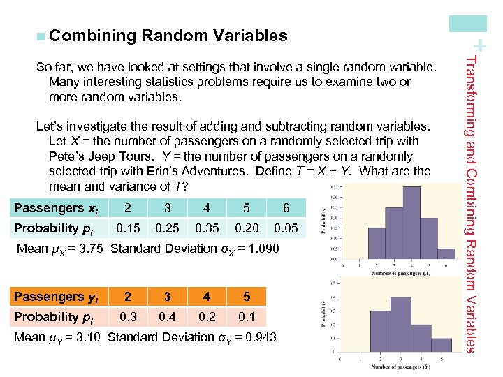
Random Variables Let’s investigate the result of adding and subtracting random variables. Let X = the number of passengers on a randomly selected trip with Pete’s Jeep Tours. Y = the number of passengers on a randomly selected trip with Erin’s Adventures. Define T = X + Y. What are the mean and variance of T? Passengers xi 2 3 4 5 6 Probability pi 0. 15 0. 25 0. 35 0. 20 0. 05 Mean µX = 3. 75 Standard Deviation σX = 1. 090 Passengers yi 2 3 4 5 Probability pi 0. 3 0. 4 0. 2 0. 1 Mean µY = 3. 10 Standard Deviation σY = 0. 943 Transforming and Combining Random Variables So far, we have looked at settings that involve a single random variable. Many interesting statistics problems require us to examine two or more random variables. + n Combining
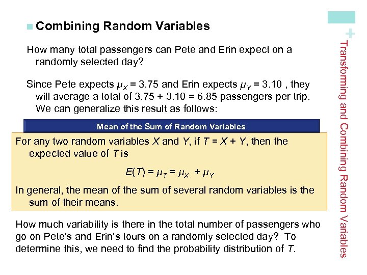
Random Variables Since Pete expects µX = 3. 75 and Erin expects µY = 3. 10 , they will average a total of 3. 75 + 3. 10 = 6. 85 passengers per trip. We can generalize this result as follows: Mean of the Sum of Random Variables For any two random variables X and Y, if T = X + Y, then the expected value of T is E(T) = µT = µX + µY In general, the mean of the sum of several random variables is the sum of their means. How much variability is there in the total number of passengers who go on Pete’s and Erin’s tours on a randomly selected day? To determine this, we need to find the probability distribution of T. Transforming and Combining Random Variables How many total passengers can Pete and Erin expect on a randomly selected day? + n Combining
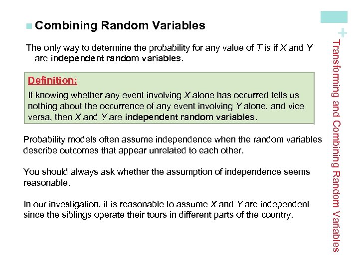
Random Variables Definition: If knowing whether any event involving X alone has occurred tells us nothing about the occurrence of any event involving Y alone, and vice versa, then X and Y are independent random variables. Probability models often assume independence when the random variables describe outcomes that appear unrelated to each other. You should always ask whether the assumption of independence seems reasonable. In our investigation, it is reasonable to assume X and Y are independent since the siblings operate their tours in different parts of the country. Transforming and Combining Random Variables The only way to determine the probability for any value of T is if X and Y are independent random variables. + n Combining
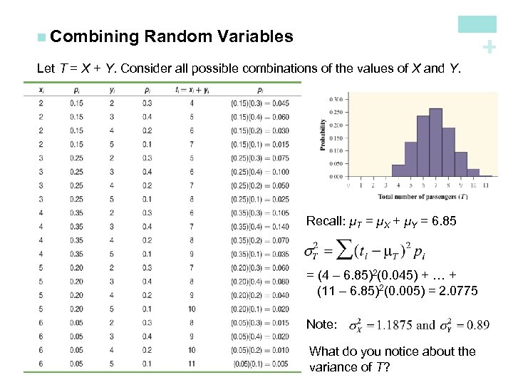
Random Variables + n Combining Let T = X + Y. Consider all possible combinations of the values of X and Y. Recall: µT = µX + µY = 6. 85 = (4 – 6. 85)2(0. 045) + … + (11 – 6. 85)2(0. 005) = 2. 0775 Note: What do you notice about the variance of T?
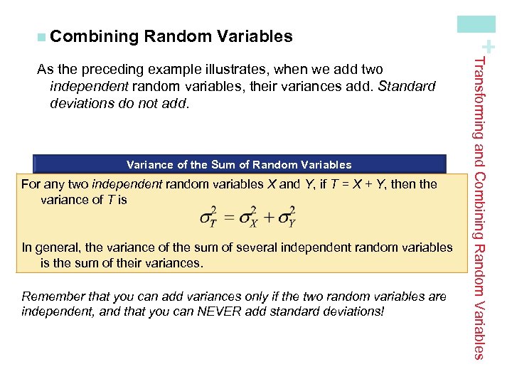
Random Variables Variance of the Sum of Random Variables For any two independent random variables X and Y, if T = X + Y, then the variance of T is In general, the variance of the sum of several independent random variables is the sum of their variances. Remember that you can add variances only if the two random variables are independent, and that you can NEVER add standard deviations! Transforming and Combining Random Variables As the preceding example illustrates, when we add two independent random variables, their variances add. Standard deviations do not add. + n Combining
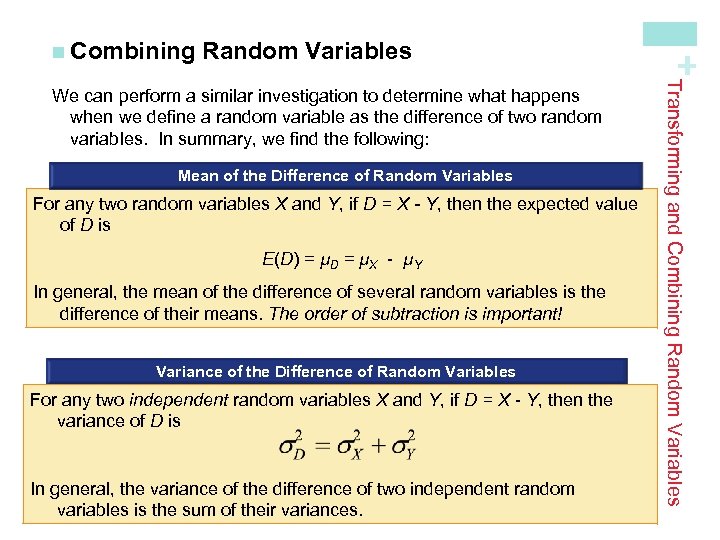
Random Variables Mean of the Difference of Random Variables For any two random variables X and Y, if D = X - Y, then the expected value of D is E(D) = µD = µX - µY In general, the mean of the difference of several random variables is the difference of their means. The order of subtraction is important! Variance of the Difference of Random Variables For any two independent random variables X and Y, if D = X - Y, then the variance of D is In general, the variance of the difference of two independent random variables is the sum of their variances. Transforming and Combining Random Variables We can perform a similar investigation to determine what happens when we define a random variable as the difference of two random variables. In summary, we find the following: + n Combining
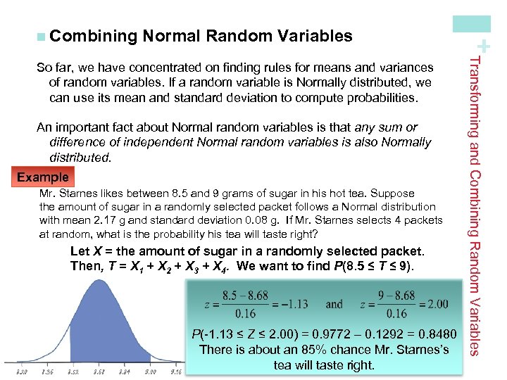
Normal Random Variables An important fact about Normal random variables is that any sum or difference of independent Normal random variables is also Normally distributed. Example Mr. Starnes likes between 8. 5 and 9 grams of sugar in his hot tea. Suppose the amount of sugar in a randomly selected packet follows a Normal distribution with mean 2. 17 g and standard deviation 0. 08 g. If Mr. Starnes selects 4 packets at random, what is the probability his tea will taste right? Let X = the amount of sugar in a randomly selected packet. Then, T = X 1 + X 2 + X 3 + X 4. We want to find P(8. 5 ≤ T ≤ 9). µT = µX 1 + µX 2 + µX 3 + µX 4 = 2. 17 +2. 17 = 8. 68 P(-1. 13 ≤ Z ≤ 2. 00) = 0. 9772 – 0. 1292 = 0. 8480 There is about an 85% chance Mr. Starnes’s tea will taste right. Transforming and Combining Random Variables So far, we have concentrated on finding rules for means and variances of random variables. If a random variable is Normally distributed, we can use its mean and standard deviation to compute probabilities. + n Combining
+ Binomial and Geometric Random Variables Learning Objectives After this section, you should be able to… ü DETERMINE whether the conditions for a binomial setting are met ü COMPUTE and INTERPRET probabilities involving binomial random variables ü CALCULATE the mean and standard deviation of a binomial random variable and INTERPRET these values in context ü CALCULATE probabilities involving geometric random variables
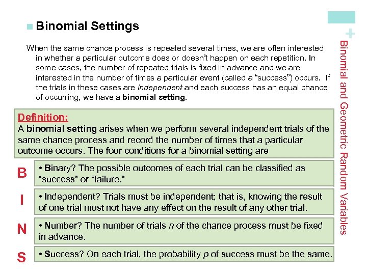
Settings Definition: A binomial setting arises when we perform several independent trials of the same chance process and record the number of times that a particular outcome occurs. The four conditions for a binomial setting are B • Binary? The possible outcomes of each trial can be classified as “success” or “failure. ” I • Independent? Trials must be independent; that is, knowing the result of one trial must not have any effect on the result of any other trial. N • Number? The number of trials n of the chance process must be fixed in advance. S • Success? On each trial, the probability p of success must be the same. Binomial and Geometric Random Variables When the same chance process is repeated several times, we are often interested in whether a particular outcome does or doesn’t happen on each repetition. In some cases, the number of repeated trials is fixed in advance and we are interested in the number of times a particular event (called a “success”) occurs. If the trials in these cases are independent and each success has an equal chance of occurring, we have a binomial setting. + n Binomial
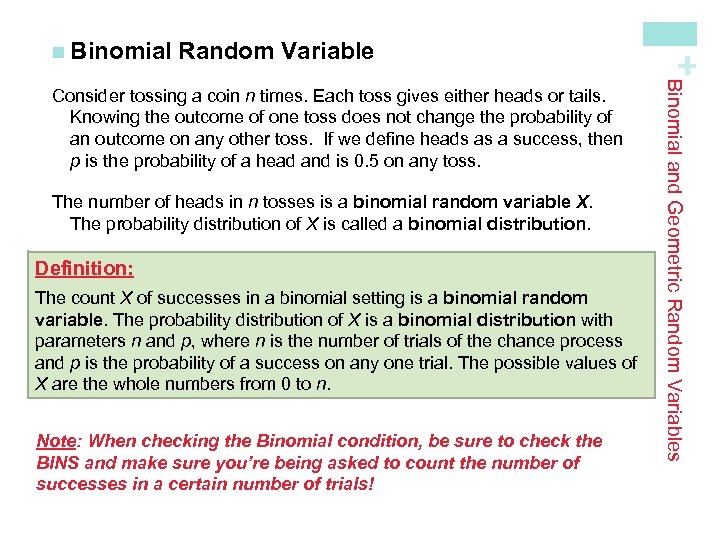
Random Variable The number of heads in n tosses is a binomial random variable X. The probability distribution of X is called a binomial distribution. Definition: The count X of successes in a binomial setting is a binomial random variable. The probability distribution of X is a binomial distribution with parameters n and p, where n is the number of trials of the chance process and p is the probability of a success on any one trial. The possible values of X are the whole numbers from 0 to n. Note: When checking the Binomial condition, be sure to check the BINS and make sure you’re being asked to count the number of successes in a certain number of trials! Binomial and Geometric Random Variables Consider tossing a coin n times. Each toss gives either heads or tails. Knowing the outcome of one toss does not change the probability of an outcome on any other toss. If we define heads as a success, then p is the probability of a head and is 0. 5 on any toss. + n Binomial
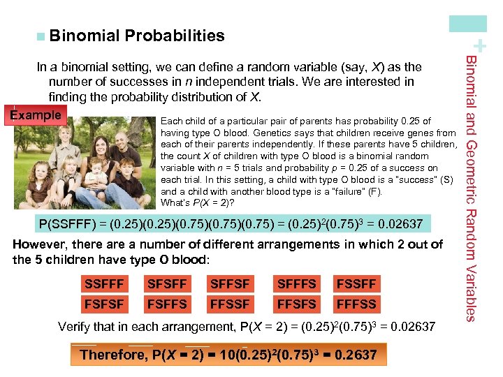
Probabilities + n Binomial having type O blood. Genetics says that children receive genes from each of their parents independently. If these parents have 5 children, the count X of children with type O blood is a binomial random variable with n = 5 trials and probability p = 0. 25 of a success on each trial. In this setting, a child with type O blood is a “success” (S) and a child with another blood type is a “failure” (F). What’s P(X = 2)? P(SSFFF) = (0. 25)(0. 75)(0. 75) = (0. 25)2(0. 75)3 = 0. 02637 However, there a number of different arrangements in which 2 out of the 5 children have type O blood: SSFFF SFSFF SFFSF SFFFS FSSFF FSFSF FSFFS FFSSF FFSFS FFFSS Verify that in each arrangement, P(X = 2) = (0. 25)2(0. 75)3 = 0. 02637 Therefore, P(X = 2) = 10(0. 25)2(0. 75)3 = 0. 2637 Binomial and Geometric Random Variables In a binomial setting, we can define a random variable (say, X) as the number of successes in n independent trials. We are interested in finding the probability distribution of X. Example Each child of a particular pair of parents has probability 0. 25 of
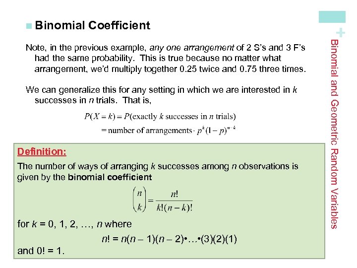
Coefficient We can generalize this for any setting in which we are interested in k successes in n trials. That is, Definition: The number of ways of arranging k successes among n observations is given by the binomial coefficient for k = 0, 1, 2, …, n where n! = n(n – 1)(n – 2) • … • (3)(2)(1) and 0! = 1. Binomial and Geometric Random Variables Note, in the previous example, any one arrangement of 2 S’s and 3 F’s had the same probability. This is true because no matter what arrangement, we’d multiply together 0. 25 twice and 0. 75 three times. + n Binomial
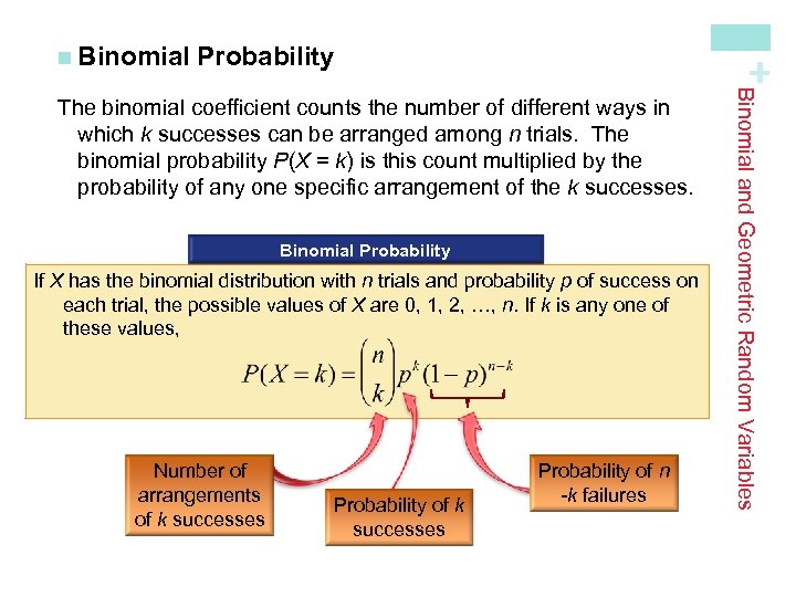
Probability + n Binomial Probability If X has the binomial distribution with n trials and probability p of success on each trial, the possible values of X are 0, 1, 2, …, n. If k is any one of these values, Number of arrangements of k successes Probability of n -k failures Binomial and Geometric Random Variables The binomial coefficient counts the number of different ways in which k successes can be arranged among n trials. The binomial probability P(X = k) is this count multiplied by the probability of any one specific arrangement of the k successes.
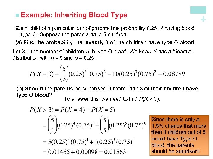
Inheriting Blood Type + n Example: Each child of a particular pair of parents has probability 0. 25 of having blood type O. Suppose the parents have 5 children (a) Find the probability that exactly 3 of the children have type O blood. Let X = the number of children with type O blood. We know X has a binomial distribution with n = 5 and p = 0. 25. (b) Should the parents be surprised if more than 3 of their children have type O blood? To answer this, we need to find P(X > 3). Since there is only a 1. 5% chance that more than 3 children out of 5 would have Type O blood, the parents should be surprised!
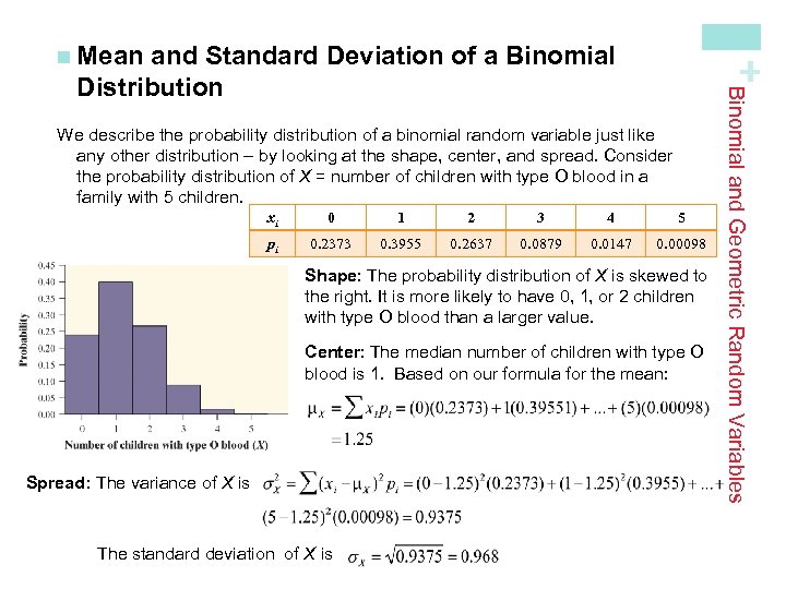
and Standard Deviation of a Binomial Distribution + n Mean xi 0 1 2 3 4 5 pi 0. 2373 0. 3955 0. 2637 0. 0879 0. 0147 0. 00098 Shape: The probability distribution of X is skewed to the right. It is more likely to have 0, 1, or 2 children with type O blood than a larger value. Center: The median number of children with type O blood is 1. Based on our formula for the mean: Spread: The variance of X is The standard deviation of X is Binomial and Geometric Random Variables We describe the probability distribution of a binomial random variable just like any other distribution – by looking at the shape, center, and spread. Consider the probability distribution of X = number of children with type O blood in a family with 5 children.
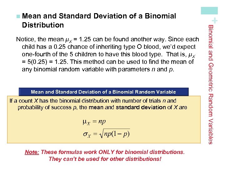
Notice, the mean µX = 1. 25 can be found another way. Since each child has a 0. 25 chance of inheriting type O blood, we’d expect one-fourth of the 5 children to have this blood type. That is, µX = 5(0. 25) = 1. 25. This method can be used to find the mean of any binomial random variable with parameters n and p. Mean and Standard Deviation of a Binomial Random Variable If a count X has the binomial distribution with number of trials n and probability of success p, the mean and standard deviation of X are Note: These formulas work ONLY for binomial distributions. They can’t be used for other distributions! Binomial and Geometric Random Variables and Standard Deviation of a Binomial Distribution + n Mean
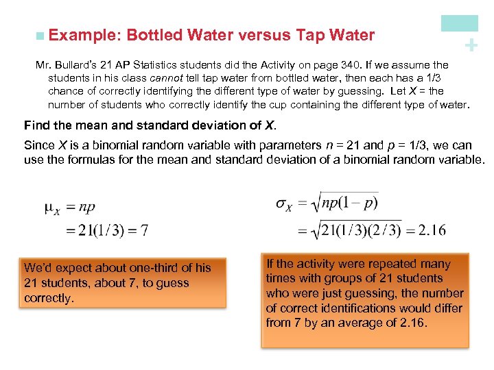
Bottled Water versus Tap Water + n Example: Mr. Bullard’s 21 AP Statistics students did the Activity on page 340. If we assume the students in his class cannot tell tap water from bottled water, then each has a 1/3 chance of correctly identifying the different type of water by guessing. Let X = the number of students who correctly identify the cup containing the different type of water. Find the mean and standard deviation of X. Since X is a binomial random variable with parameters n = 21 and p = 1/3, we can use the formulas for the mean and standard deviation of a binomial random variable. We’d expect about one-third of his 21 students, about 7, to guess correctly. If the activity were repeated many times with groups of 21 students who were just guessing, the number of correct identifications would differ from 7 by an average of 2. 16.
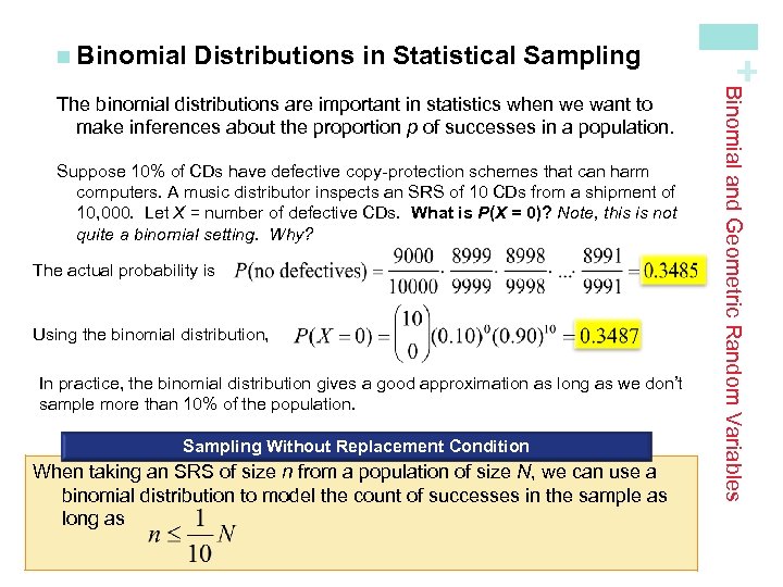
Distributions in Statistical Sampling Suppose 10% of CDs have defective copy-protection schemes that can harm computers. A music distributor inspects an SRS of 10 CDs from a shipment of 10, 000. Let X = number of defective CDs. What is P(X = 0)? Note, this is not quite a binomial setting. Why? The actual probability is Using the binomial distribution, In practice, the binomial distribution gives a good approximation as long as we don’t sample more than 10% of the population. Sampling Without Replacement Condition When taking an SRS of size n from a population of size N, we can use a binomial distribution to model the count of successes in the sample as long as Binomial and Geometric Random Variables The binomial distributions are important in statistics when we want to make inferences about the proportion p of successes in a population. + n Binomial
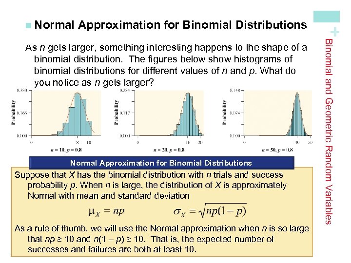
Approximation for Binomial Distributions Normal Approximation for Binomial Distributions Suppose that X has the binomial distribution with n trials and success probability p. When n is large, the distribution of X is approximately Normal with mean and standard deviation As a rule of thumb, we will use the Normal approximation when n is so large that np ≥ 10 and n(1 – p) ≥ 10. That is, the expected number of successes and failures are both at least 10. Binomial and Geometric Random Variables As n gets larger, something interesting happens to the shape of a binomial distribution. The figures below show histograms of binomial distributions for different values of n and p. What do you notice as n gets larger? + n Normal
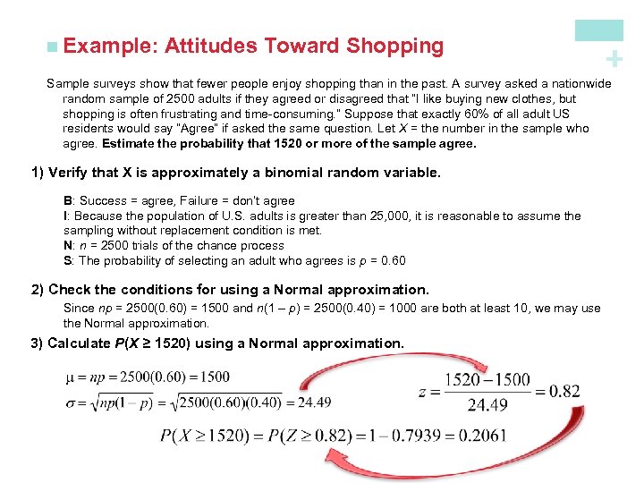
Attitudes Toward Shopping + n Example: Sample surveys show that fewer people enjoy shopping than in the past. A survey asked a nationwide random sample of 2500 adults if they agreed or disagreed that “I like buying new clothes, but shopping is often frustrating and time-consuming. ” Suppose that exactly 60% of all adult US residents would say “Agree” if asked the same question. Let X = the number in the sample who agree. Estimate the probability that 1520 or more of the sample agree. 1) Verify that X is approximately a binomial random variable. B: Success = agree, Failure = don’t agree I: Because the population of U. S. adults is greater than 25, 000, it is reasonable to assume the sampling without replacement condition is met. N: n = 2500 trials of the chance process S: The probability of selecting an adult who agrees is p = 0. 60 2) Check the conditions for using a Normal approximation. Since np = 2500(0. 60) = 1500 and n(1 – p) = 2500(0. 40) = 1000 are both at least 10, we may use the Normal approximation. 3) Calculate P(X ≥ 1520) using a Normal approximation.
Settings Definition: A geometric setting arises when we perform independent trials of the same chance process and record the number of trials until a particular outcome occurs. The four conditions for a geometric setting are B • Binary? The possible outcomes of each trial can be classified as “success” or “failure. ” I • Independent? Trials must be independent; that is, knowing the result of one trial must not have any effect on the result of any other trial. T • Trials? The goal is to count the number of trials until the first success occurs. S • Success? On each trial, the probability p of success must be the same. Binomial and Geometric Random Variables In a binomial setting, the number of trials n is fixed and the binomial random variable X counts the number of successes. In other situations, the goal is to repeat a chance behavior until a success occurs. These situations are called geometric settings. + n Geometric
Random Variable Definition: The number of trials Y that it takes to get a success in a geometric setting is a geometric random variable. The probability distribution of Y is a geometric distribution with parameter p, the probability of a success on any trial. The possible values of Y are 1, 2, 3, …. Note: Like binomial random variables, it is important to be able to distinguish situations in which the geometric distribution does and doesn’t apply! Binomial and Geometric Random Variables In a geometric setting, if we define the random variable Y to be the number of trials needed to get the first success, then Y is called a geometric random variable. The probability distribution of Y is called a geometric distribution. + n Geometric
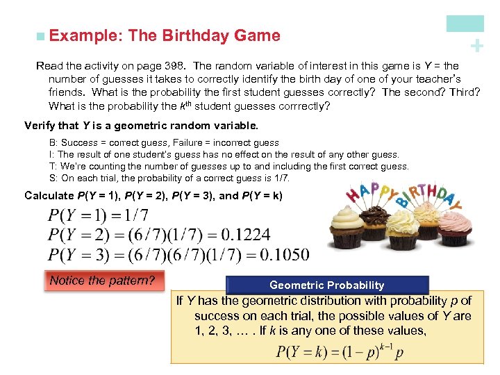
The Birthday Game + n Example: Read the activity on page 398. The random variable of interest in this game is Y = the number of guesses it takes to correctly identify the birth day of one of your teacher’s friends. What is the probability the first student guesses correctly? The second? Third? What is the probability the kth student guesses corrrectly? Verify that Y is a geometric random variable. B: Success = correct guess, Failure = incorrect guess I: The result of one student’s guess has no effect on the result of any other guess. T: We’re counting the number of guesses up to and including the first correct guess. S: On each trial, the probability of a correct guess is 1/7. Calculate P(Y = 1), P(Y = 2), P(Y = 3), and P(Y = k) Notice the pattern? Geometric Probability If Y has the geometric distribution with probability p of success on each trial, the possible values of Y are 1, 2, 3, …. If k is any one of these values,
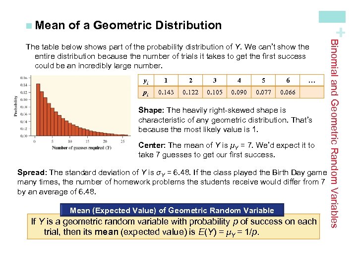
of a Geometric Distribution + n Mean yi 1 2 3 4 5 6 pi 0. 143 0. 122 0. 105 0. 090 0. 077 … 0. 066 Shape: The heavily right-skewed shape is characteristic of any geometric distribution. That’s because the most likely value is 1. Center: The mean of Y is µY = 7. We’d expect it to take 7 guesses to get our first success. Spread: The standard deviation of Y is σY = 6. 48. If the class played the Birth Day game many times, the number of homework problems the students receive would differ from 7 by an average of 6. 48. Mean (Expected Value) of Geometric Random Variable If Y is a geometric random variable with probability p of success on each trial, then its mean (expected value) is E(Y) = µY = 1/p. Binomial and Geometric Random Variables The table below shows part of the probability distribution of Y. We can’t show the entire distribution because the number of trials it takes to get the first success could be an incredibly large number.
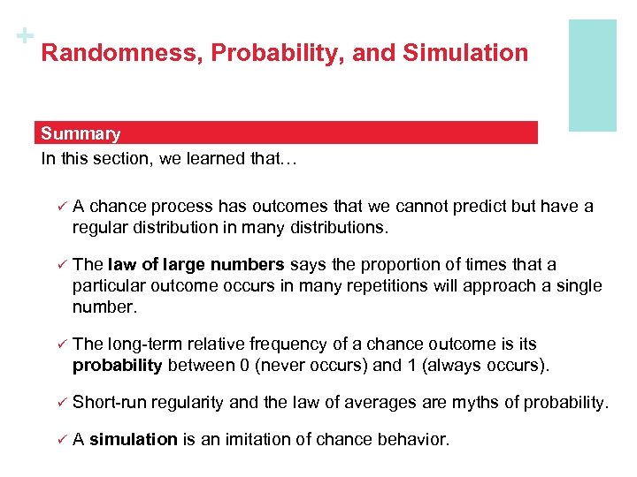
+ Randomness, Probability, and Simulation Summary In this section, we learned that… ü A chance process has outcomes that we cannot predict but have a regular distribution in many distributions. ü The law of large numbers says the proportion of times that a particular outcome occurs in many repetitions will approach a single number. ü The long-term relative frequency of a chance outcome is its probability between 0 (never occurs) and 1 (always occurs). ü Short-run regularity and the law of averages are myths of probability. ü A simulation is an imitation of chance behavior.
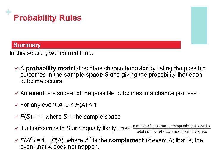
+ Probability Rules Summary In this section, we learned that… ü A probability model describes chance behavior by listing the possible outcomes in the sample space S and giving the probability that each outcome occurs. ü An event is a subset of the possible outcomes in a chance process. ü For any event A, 0 ≤ P(A) ≤ 1 ü P(S) = 1, where S = the sample space ü If all outcomes in S are equally likely, ü P(AC) = 1 – P(A), where AC is the complement of event A; that is, the event that A does not happen.
+ Probability Rules Summary In this section, we learned that… ü Events A and B are mutually exclusive (disjoint) if they have no outcomes in common. If A and B are disjoint, P(A or B) = P(A) + P(B). ü A two-way table or a Venn diagram can be used to display the sample space for a chance process. ü The intersection (A ∩ B) of events A and B consists of outcomes in both A and B. ü The union (A ∪ B) of events A and B consists of all outcomes in event A, event B, or both. ü The general addition rule can be used to find P(A or B): P(A or B) = P(A) + P(B) – P(A and B)
+ Conditional Probability and Independence Summary In this section, we learned that… ü If one event has happened, the chance that another event will happen is a conditional probability. P(B|A) represents the probability that event B occurs given that event A has occurred. ü Events A and B are independent if the chance that event B occurs is not affected by whether event A occurs. If two events are mutually exclusive (disjoint), they cannot be independent. ü When chance behavior involves a sequence of outcomes, a tree diagram can be used to describe the sample space. ü The general multiplication rule states that the probability of events A and B occurring together is P(A ∩ B)=P(A) • P(B|A) ü In the special case of independent events, P(A ∩ B)=P(A) • P(B) ü The conditional probability formula states P(B|A) = P(A ∩ B) / P(A)
+ Discrete and Continuous Random Variables Summary In this section, we learned that… ü A random variable is a variable taking numerical values determined by the outcome of a chance process. The probability distribution of a random variable X tells us what the possible values of X are and how probabilities are assigned to those values. ü A discrete random variable has a fixed set of possible values with gaps between them. The probability distribution assigns each of these values a probability between 0 and 1 such that the sum of all the probabilities is exactly 1. ü A continuous random variable takes all values in some interval of numbers. A density curve describes the probability distribution of a continuous random variable.
+ Discrete and Continuous Random Variables Summary In this section, we learned that… ü The mean of a random variable is the long-run average value of the variable after many repetitions of the chance process. It is also known as the expected value of the random variable. ü The expected value of a discrete random variable X is ü The variance of a random variable is the average squared deviation of the values of the variable from their mean. The standard deviation is the square root of the variance. For a discrete random variable X,
+ Transforming and Combining Random Variables Summary In this section, we learned that… ü Adding a constant a (which could be negative) to a random variable increases (or decreases) the mean of the random variable by a but does not affect its standard deviation or the shape of its probability distribution. ü Multiplying a random variable by a constant b (which could be negative) multiplies the mean of the random variable by b and the standard deviation by |b| but does not change the shape of its probability distribution. ü A linear transformation of a random variable involves adding a constant a, multiplying by a constant b, or both. If we write the linear transformation of X in the form Y = a + b. X, the following about are true about Y: ü Shape: same as the probability distribution of X. ü Center: µY = a + bµX ü Spread: σY = |b|σX
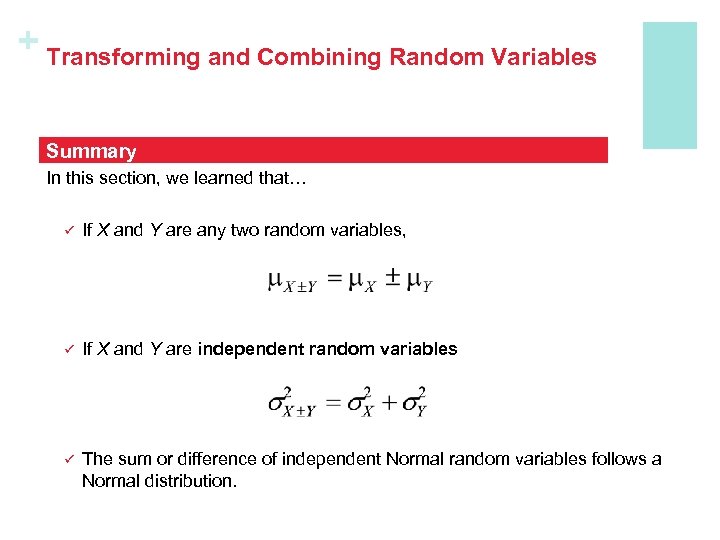
+ Transforming and Combining Random Variables Summary In this section, we learned that… ü If X and Y are any two random variables, ü If X and Y are independent random variables ü The sum or difference of independent Normal random variables follows a Normal distribution.
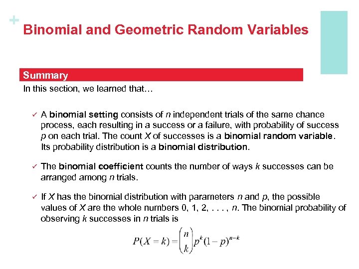
+ Binomial and Geometric Random Variables Summary In this section, we learned that… ü A binomial setting consists of n independent trials of the same chance process, each resulting in a success or a failure, with probability of success p on each trial. The count X of successes is a binomial random variable. Its probability distribution is a binomial distribution. ü The binomial coefficient counts the number of ways k successes can be arranged among n trials. ü If X has the binomial distribution with parameters n and p, the possible values of X are the whole numbers 0, 1, 2, . . . , n. The binomial probability of observing k successes in n trials is
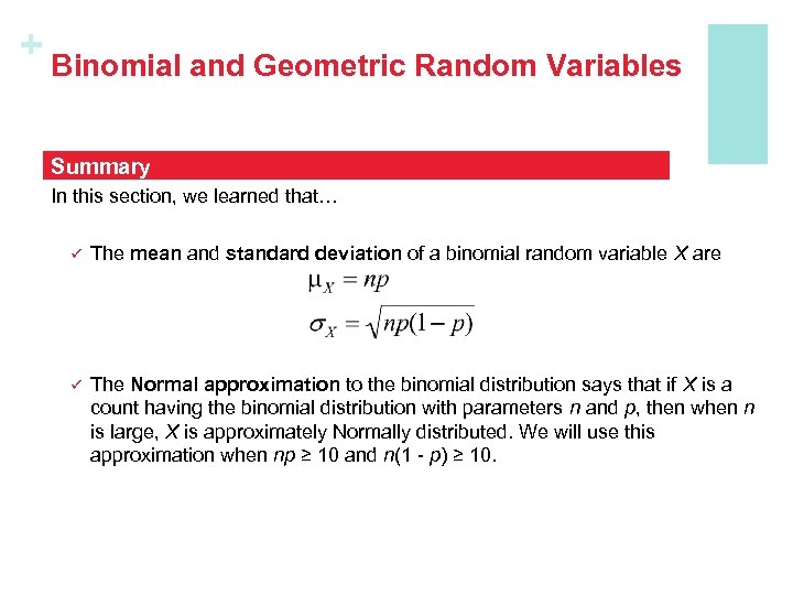
+ Binomial and Geometric Random Variables Summary In this section, we learned that… ü The mean and standard deviation of a binomial random variable X are ü The Normal approximation to the binomial distribution says that if X is a count having the binomial distribution with parameters n and p, then when n is large, X is approximately Normally distributed. We will use this approximation when np ≥ 10 and n(1 - p) ≥ 10.
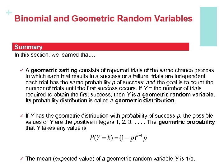
+ Binomial and Geometric Random Variables Summary In this section, we learned that… ü A geometric setting consists of repeated trials of the same chance process in which each trial results in a success or a failure; trials are independent; each trial has the same probability p of success; and the goal is to count the number of trials until the first success occurs. If Y = the number of trials required to obtain the first success, then Y is a geometric random variable. Its probability distribution is called a geometric distribution. ü If Y has the geometric distribution with probability of success p, the possible values of Y are the positive integers 1, 2, 3, . . The geometric probability that Y takes any value is ü The mean (expected value) of a geometric random variable Y is 1/p.
3a51e6eb3073412be00eb586a86ec92c.ppt