Probability Models in Marketing Marketing models attempt

Probability Models in Marketing • Marketing models attempt to describe or predict behaviour – Usually include a random element to allow for imperfect knowledge • We will develop probability models that specify a random model for individual behaviour – Sum this across individuals to get a model of aggregate measures – May need to incorporate differences between individuals into the model

Uses of Probability Models • Understand profile individual behaviour • Understand market-level patterns, and their origin in individual behaviours • Provide norms or benchmarks for comparison – Ehrenburg: Understanding Buyer Behaviour; and Repeat-Buying (1988) – Latter book available free online at http: //www. empgens. com/ehrenberg. html#repeat • Prediction or forecasting of: – Aggregate results beyond current observation period – Individual behaviour, given knowledge of past actions

Product Trial Example • Have a newly launched product – Multi-pack juice drink, aimed at children – Launched in test market – May be rolled out nationally if successful • Measure trial over time – Based on household scanner panel data, e. g. ACNielsen’s Home. Scan • Have data from first 13 weeks • Want to predict trial 13 weeks later

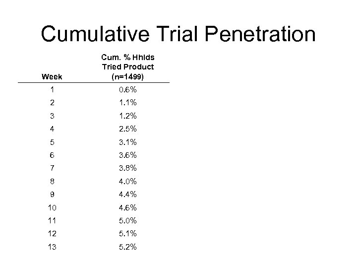
Cumulative Trial Penetration Week Cum. % Hhlds Tried Product (n=1499) 1 0. 6% 2 1. 1% 3 1. 2% 4 2. 5% 5 3. 1% 6 3. 6% 7 3. 8% 8 4. 0% 9 4. 4% 10 4. 6% 11 5. 0% 12 5. 1% 13 5. 2%

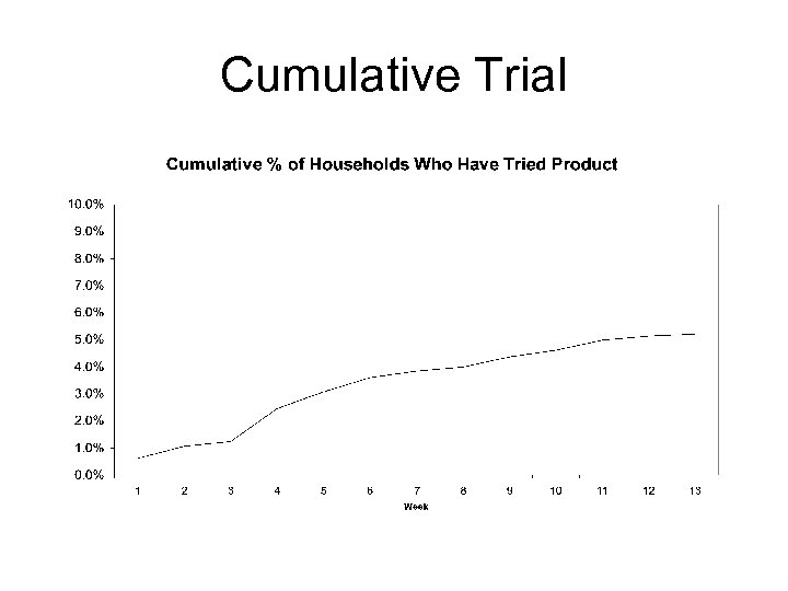
Cumulative Trial

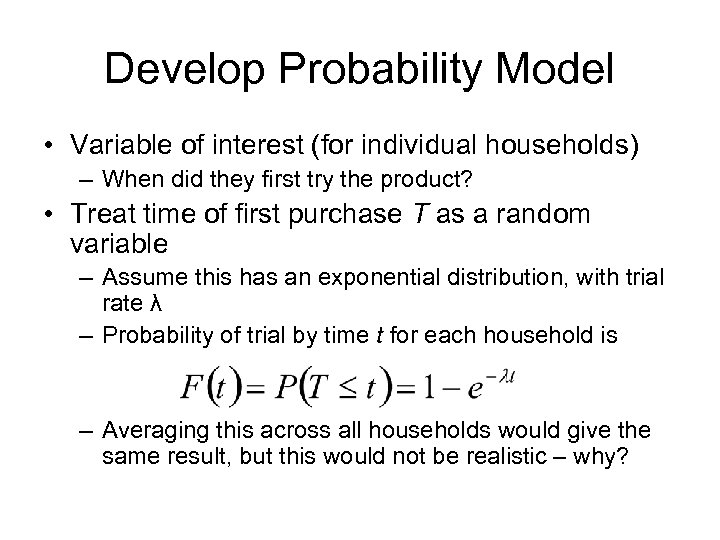
Develop Probability Model • Variable of interest (for individual households) – When did they first try the product? • Treat time of first purchase T as a random variable – Assume this has an exponential distribution, with trial rate λ – Probability of trial by time t for each household is – Averaging this across all households would give the same result, but this would not be realistic – why?

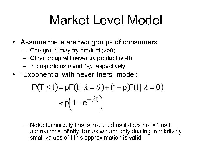
Market Level Model • Assume there are two groups of consumers – One group may try product (λ>0) – Other group will never try product (λ~0) – In proportions p and 1 -p respectively • “Exponential with never-triers” model: – Note: technically this is not a cdf as it does not =1 as t approaches infinity, but as we are only dealing in relatively small values of t this approximation is valid.

Estimate Parameters • Model has parameters p and λ • Estimate these parameters using maximum likelihood – The likelihood function is the probability that this dataset would be observed • Viewed as a function of the parameters • Assumes the model holds • L(parameters) = P(this data observed|parameters) – The maximum likelihood estimates (MLEs) of the parameters are the values that maximise L(. ), for the given dataset – Can equivalently maximise l(. ), the log-likelihood

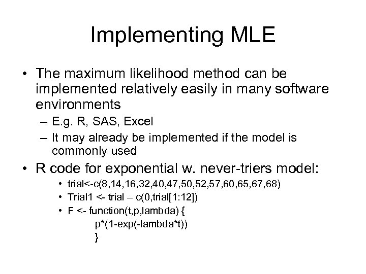
Implementing MLE • The maximum likelihood method can be implemented relatively easily in many software environments – E. g. R, SAS, Excel – It may already be implemented if the model is commonly used • R code for exponential w. never-triers model: • trial<-c(8, 14, 16, 32, 40, 47, 50, 52, 57, 60, 65, 67, 68) • Trial 1 <- trial – c(0, trial[1: 12]) • F <- function(t, p, lambda) { p*(1 -exp(-lambda*t)) }

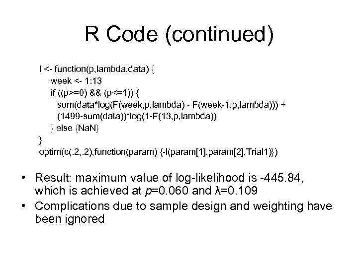
R Code (continued) l <- function(p, lambda, data) { week <- 1: 13 if ((p>=0) && (p<=1)) { sum(data*log(F(week, p, lambda) - F(week-1, p, lambda))) + (1499 -sum(data))*log(1 -F(13, p, lambda)) } else {Na. N} } optim(c(. 2, . 2), function(param) {-l(param[1], param[2], Trial 1)}) • Result: maximum value of log-likelihood is -445. 84, which is achieved at p=0. 060 and λ=0. 109 • Complications due to sample design and weighting have been ignored

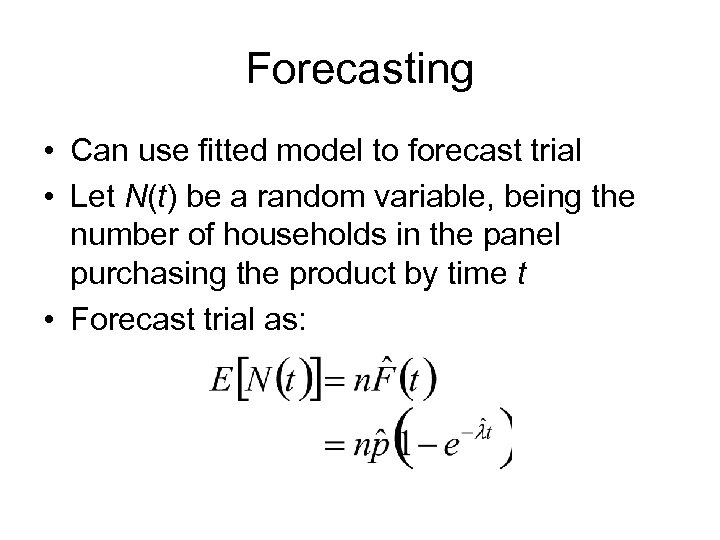
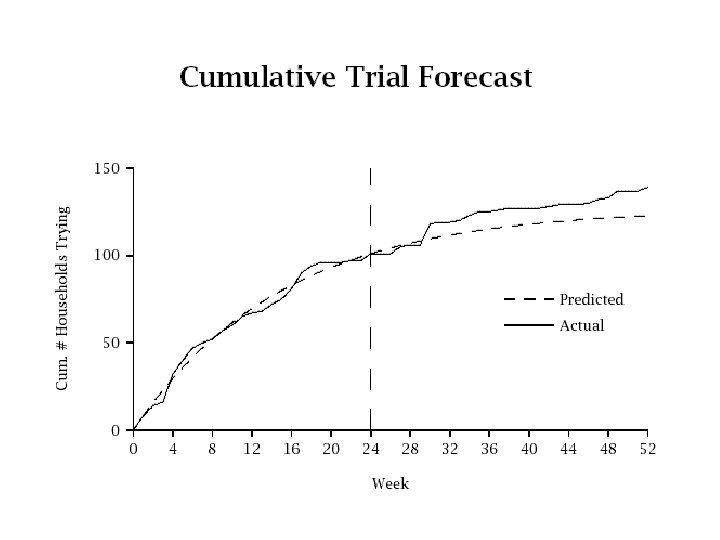
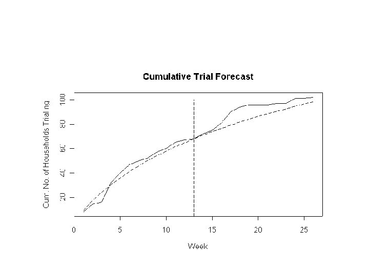
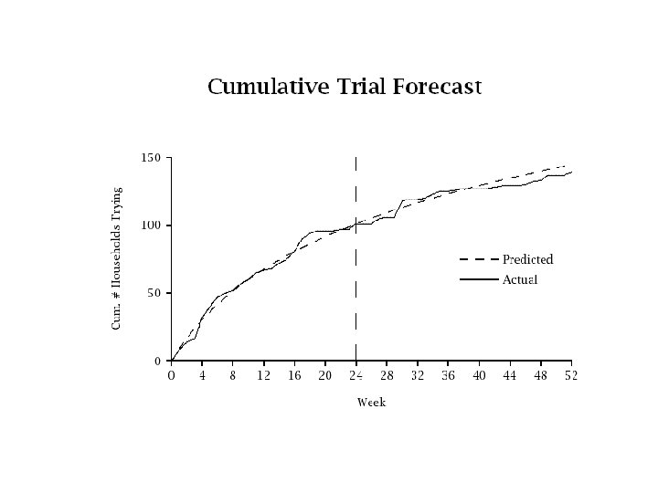
Forecasting • Can use fitted model to forecast trial • Let N(t) be a random variable, being the number of households in the panel purchasing the product by time t • Forecast trial as:

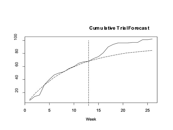
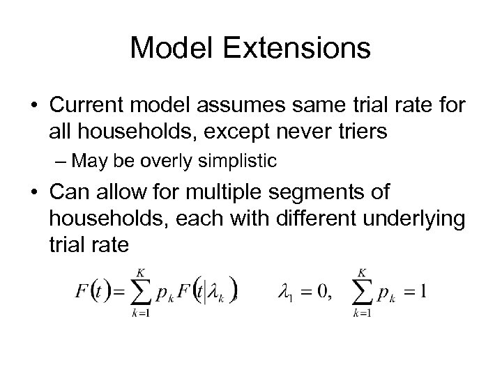
Model Extensions • Current model assumes same trial rate for all households, except never triers – May be overly simplistic • Can allow for multiple segments of households, each with different underlying trial rate

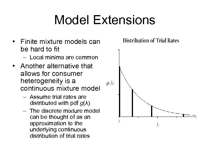
Model Extensions • Finite mixture models can be hard to fit – Local minima are common • Another alternative that allows for consumer heterogeneity is a continuous mixture model – Assume trial rates are distributed with pdf g(λ) – The discrete mixture model can be thought of as an approximation to the underlying continuous distribution of trial rates

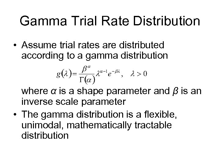
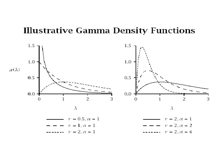
Gamma Trial Rate Distribution • Assume trial rates are distributed according to a gamma distribution where α is a shape parameter and β is an inverse scale parameter • The gamma distribution is a flexible, unimodal, mathematically tractable distribution

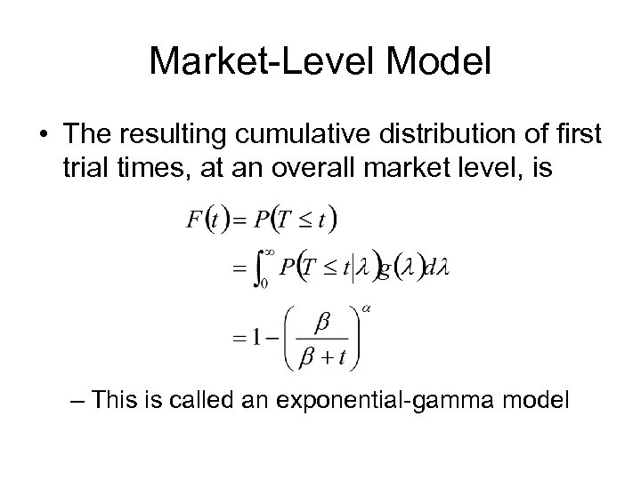
Market-Level Model • The resulting cumulative distribution of first trial times, at an overall market level, is – This is called an exponential-gamma model

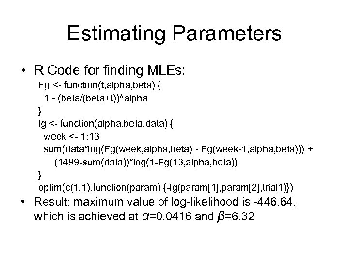
Estimating Parameters • R Code for finding MLEs: Fg <- function(t, alpha, beta) { 1 - (beta/(beta+t))^alpha } lg <- function(alpha, beta, data) { week <- 1: 13 sum(data*log(Fg(week, alpha, beta) - Fg(week-1, alpha, beta))) + (1499 -sum(data))*log(1 -Fg(13, alpha, beta)) } optim(c(1, 1), function(param) {-lg(param[1], param[2], trial 1)}) • Result: maximum value of log-likelihood is -446. 64, which is achieved at α=0. 0416 and β=6. 32

Further Extensions • Could add a “never try” component into the exponential-gamma model • Could incorporate the effects of marketing covariates – E. g. advertising weight over time • Could incorporate the effects of household covariates – E. g. presence of children

Building a Probability Model: General Approach 1. Determine the marketing problem or information needed 2. Identify the behaviour of interest at the individual level – Make sure this is observable; denote by x 3. Choose an appropriate probability distribution f(x|θ) – The parameters θ of this distribution can be thought of as latent traits of each individual • Latent or underlying traits; not observed directly but affect x

General Approach (continued) 4. Specify a distribution for the latent traits across the population – Denote this by g(θ) • • Called the mixing distribution Can be discrete, continuous or a combination 5. Obtain the resulting aggregate marketlevel distribution (if this is observed or of interest) by integrating with respect to θ

General Approach (continued) 6. Estimate the parameters of the mixing distribution – Usually done using maximum likelihood – Check model fit, graphically if possible 7. Use the fitted model to solve the marketing problem or to obtain the required information

Outdoor Advertising Example • Advertisers can buy a “monthly showing” on a set of specific billboards • Effectiveness of the showing is primarily evaluated through three measures • Reach, frequency and gross ratings points (GRPs) • Measures derived from daily travel maps filled in by a sample of people – An “exposure” is counted when a respondent goes past one of the billboards, while facing the billboard • Have data from each person for one week • Want to project from this data to get measures for the relevant month (or four weeks)

Measures of Advertising Exposure • Three measures are commonly used – Reach is the proportion of people exposed to the advertising at least once during the month – Frequency is the number of times each person is exposed to the advertising message • Usually summarised as the average frequency, which is the average number of exposures experienced among those who were exposed – Gross rating points (GRPs) is the mean number of exposures per 100 people • This is just the product of the reach (expressed as a percentage) with the average frequency

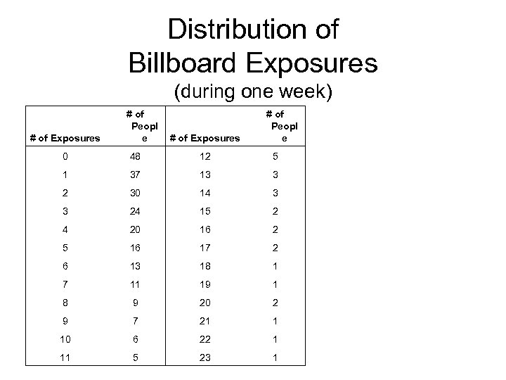
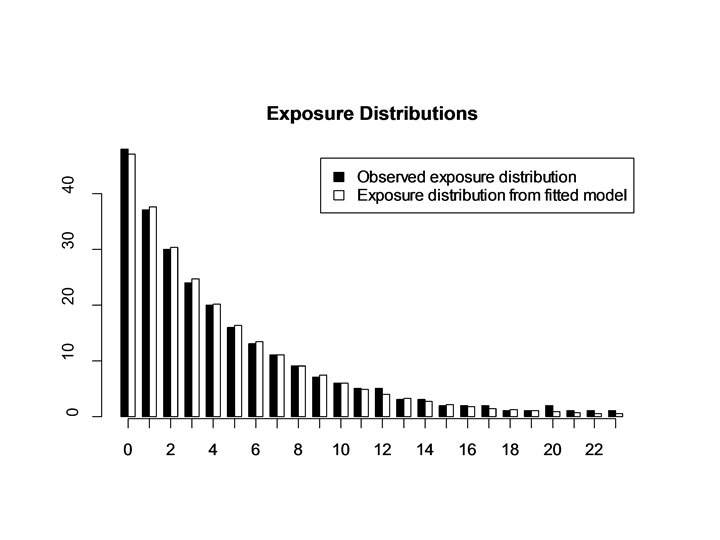
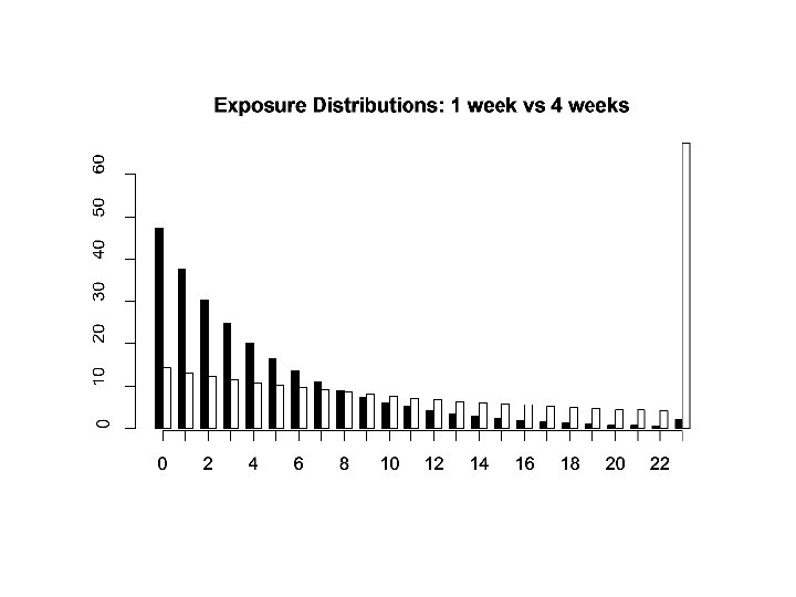
Distribution of Billboard Exposures (during one week) # of Exposures # of Peopl e 0 48 12 5 1 37 13 3 2 30 14 3 3 24 15 2 4 20 16 2 5 16 17 2 6 13 18 1 7 11 19 1 8 9 20 2 9 7 21 1 10 6 22 1 11 5 23 1

Model: Aim and Approach • Goal: Develop a model that uses one week data to provide an estimate of the monthly performance measures • Approach – Model the weekly exposure distribution – Derive the monthly exposure distribution under this model, and estimate summary statistics for the month

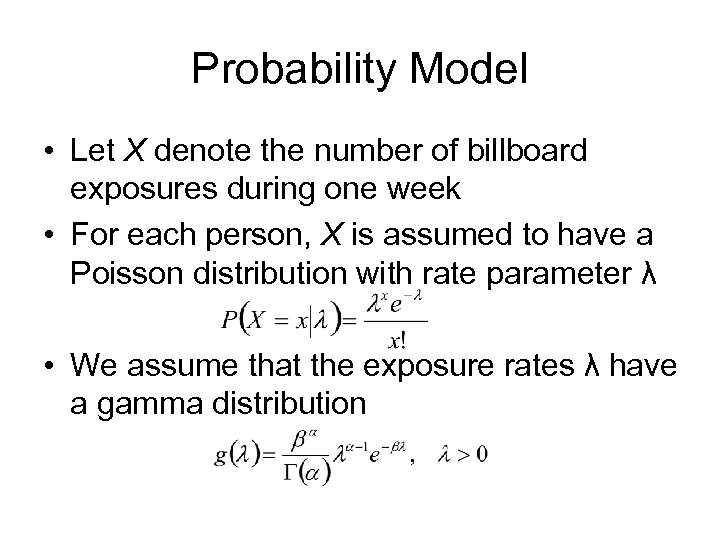
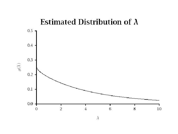
Probability Model • Let X denote the number of billboard exposures during one week • For each person, X is assumed to have a Poisson distribution with rate parameter λ • We assume that the exposure rates λ have a gamma distribution

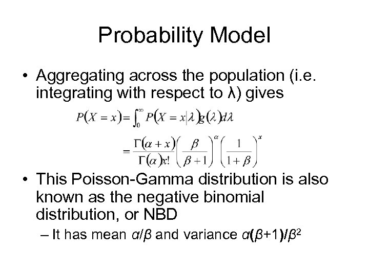
Probability Model • Aggregating across the population (i. e. integrating with respect to λ) gives • This Poisson-Gamma distribution is also known as the negative binomial distribution, or NBD – It has mean α/β and variance α(β+1)/β 2

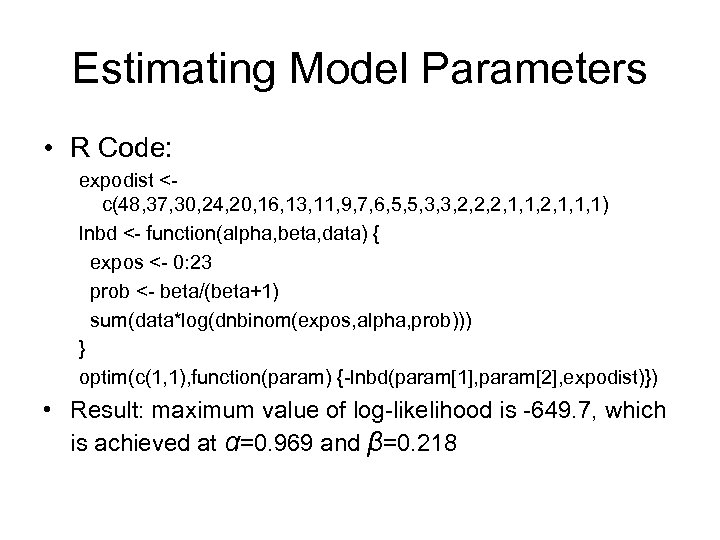
Estimating Model Parameters • R Code: expodist <- c(48, 37, 30, 24, 20, 16, 13, 11, 9, 7, 6, 5, 5, 3, 3, 2, 2, 2, 1, 1, 1) lnbd <- function(alpha, beta, data) { expos <- 0: 23 prob <- beta/(beta+1) sum(data*log(dnbinom(expos, alpha, prob))) } optim(c(1, 1), function(param) {-lnbd(param[1], param[2], expodist)}) • Result: maximum value of log-likelihood is -649. 7, which is achieved at α=0. 969 and β=0. 218

NBD For More Than 1 Week • Let X(t) denote the number of exposures experienced by a person over t weeks • Suppose that over one week, the exposure distribution for that person is Poisson(λ) • Then X(t) is also Poisson, with rate parameter λt

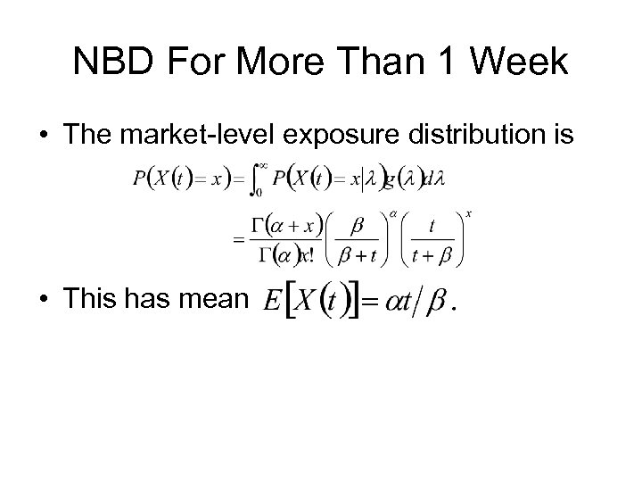
NBD For More Than 1 Week • The market-level exposure distribution is • This has mean

Performance of Monthly Showing • For t=4: – P(X(t)=0) = 0. 056 – E[X(t)] = 17. 82 • So: – Reach = 1 - P(X(t)=0) = 94. 4% – Average Frequency = E[X(t)] / (1 - P(X(t)=0) = 18. 9 – GRPs = 100* E[X(t)] =1782

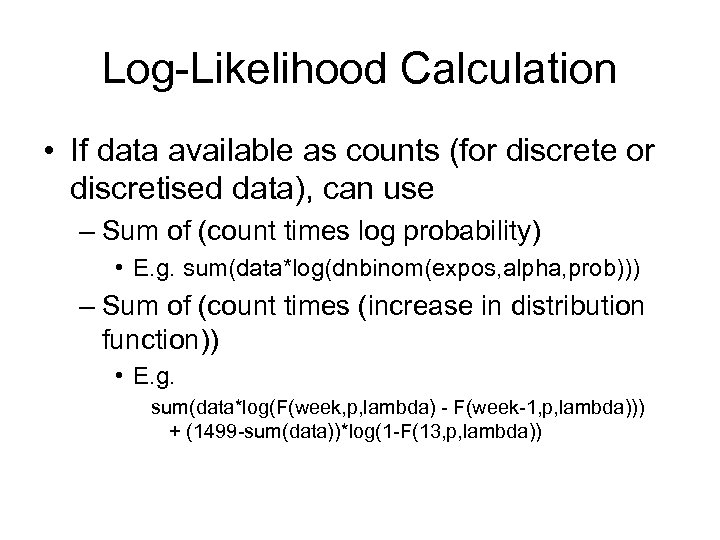
Log-Likelihood Calculation • If data available as counts (for discrete or discretised data), can use – Sum of (count times log probability) • E. g. sum(data*log(dnbinom(expos, alpha, prob))) – Sum of (count times (increase in distribution function)) • E. g. sum(data*log(F(week, p, lambda) - F(week-1, p, lambda))) + (1499 -sum(data))*log(1 -F(13, p, lambda))

Direct Marketing Example • Have customer database containing data on past purchases – 126 segments defined based on purchase histories • We’ll cover segmentation methods later • Believe that some customers are more likely to respond to mail-out than others – Send test mail-out to 3% sample of customers – Analyse response by segment to identify most profitable groups to target

Target Segments • Profitable to send mail-out if it costs less than the profit on resulting sales – i. e. if the expected rate of purchase response (PRR) is above the following cut-off: PRR > cost per letter of mail-out / unit margin – Mail-out cost is 33. 43 cents per letter – Unit margin is $161. 50 – Cut-off rate is 0. 21% • Standard approach – Conduct full mail-out to all segments with test PRR above this cut-off value – 51 segments in this case • There is a problem with this rule – what is it? • Manager chose to mail-out to 47 of these segments, plus another 24 segments

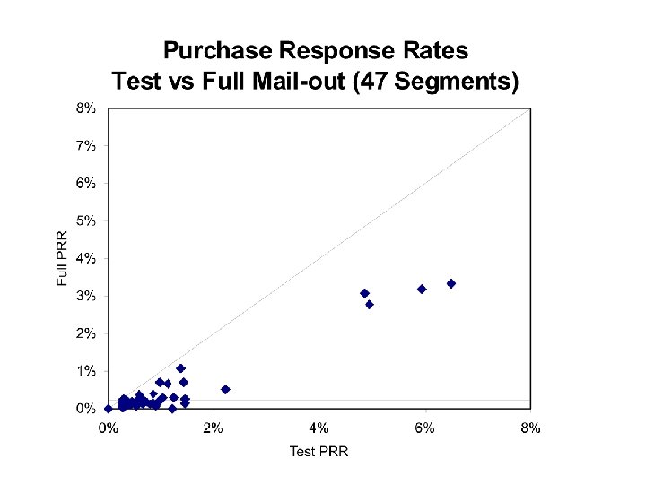
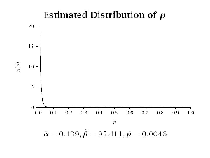
Develop Probability Model • Objective is to enable better decisions based on the test mail-out dataset • Outcome variable is the number of responses for a specified number of letters mailed, by segment • Suggests a binomial distribution

Model Development • Notation: – Ns = size of segment s (for s = 1, 2, …, S) – ms = number of test letters sent to members of segment s – Xs = number of purchases due to responses from segment s • Assume that all members of segment s have the same probability of purchase response ps, and they respond/purchase independently • Then Xs is a binomial random variable

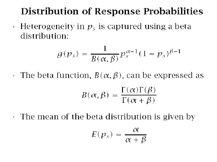
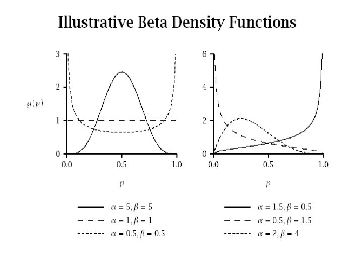
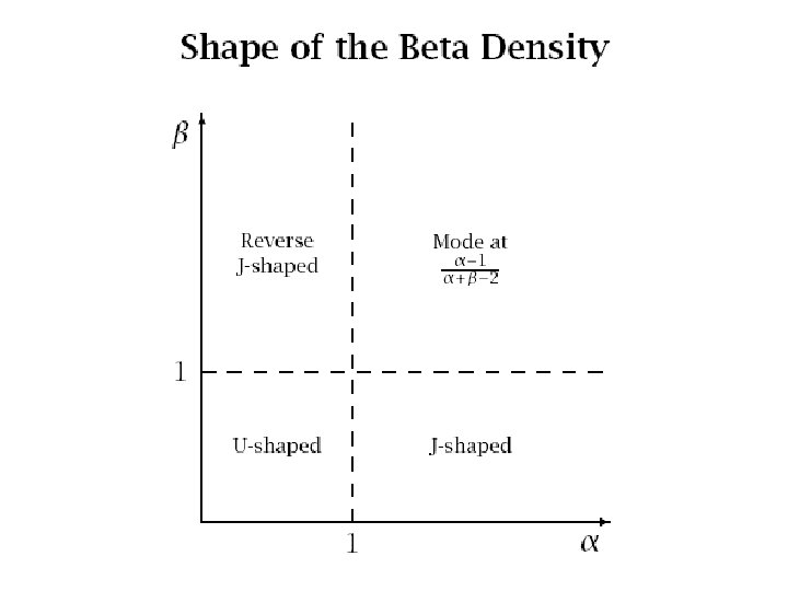
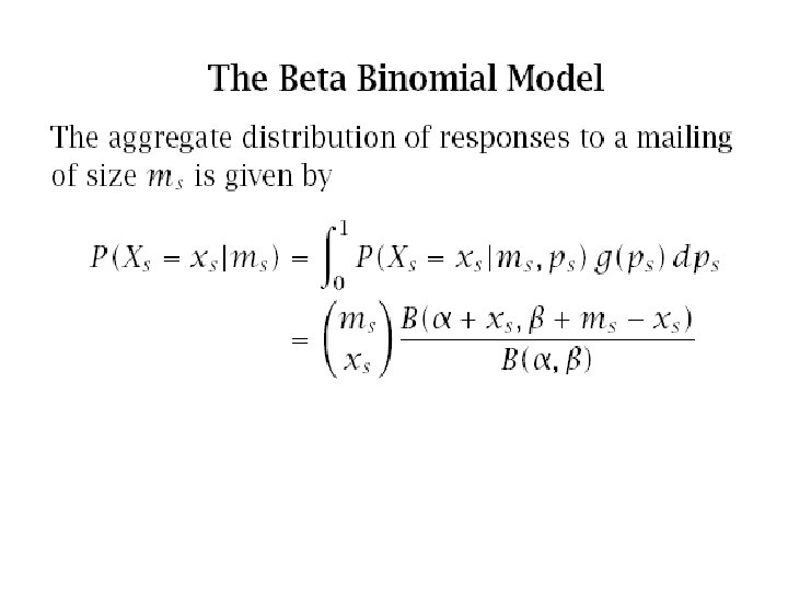
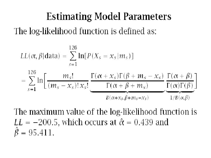
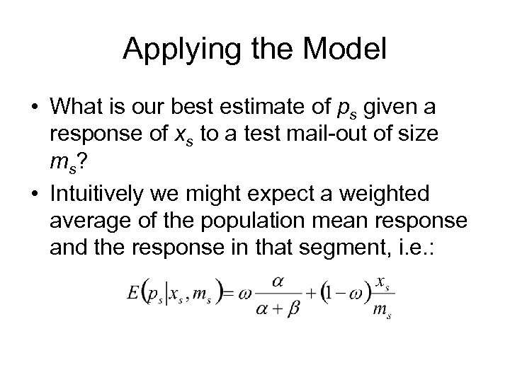
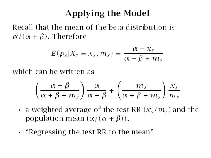
Applying the Model • What is our best estimate of ps given a response of xs to a test mail-out of size ms? • Intuitively we might expect a weighted average of the population mean response and the response in that segment, i. e. :

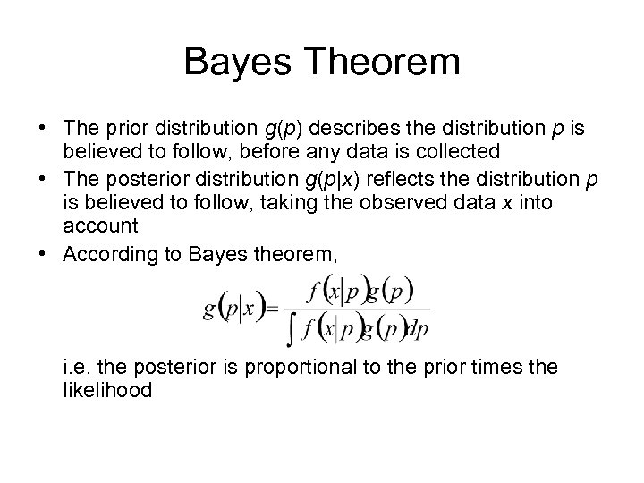
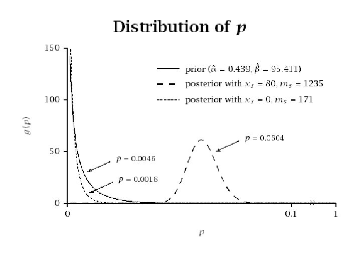
Bayes Theorem • The prior distribution g(p) describes the distribution p is believed to follow, before any data is collected • The posterior distribution g(p|x) reflects the distribution p is believed to follow, taking the observed data x into account • According to Bayes theorem, i. e. the posterior is proportional to the prior times the likelihood

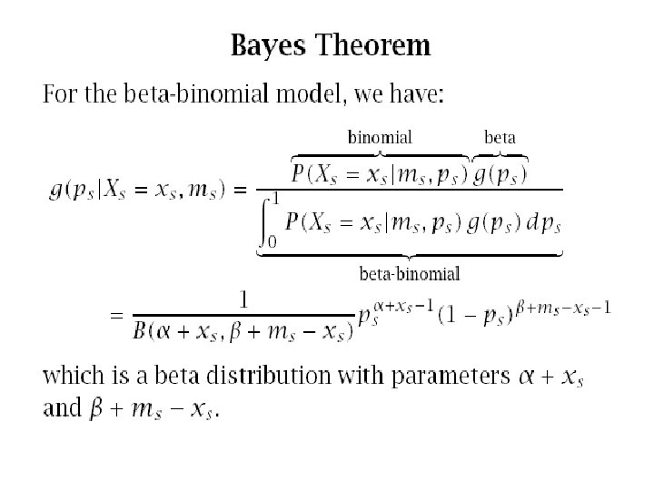
Empirical Bayes Approach • In a true Bayesian analysis, the prior distribution is specified before looking at the data • For an empirical Bayes analysis, a “prior” distribution is calculated from the data • The posterior distribution is then calculated using Bayes theorem, as on the previous slide

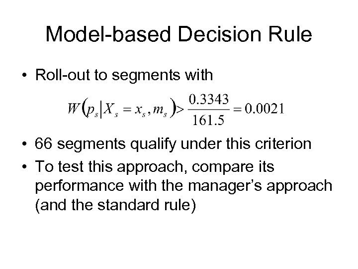
Model-based Decision Rule • Roll-out to segments with • 66 segments qualify under this criterion • To test this approach, compare its performance with the manager’s approach (and the standard rule)

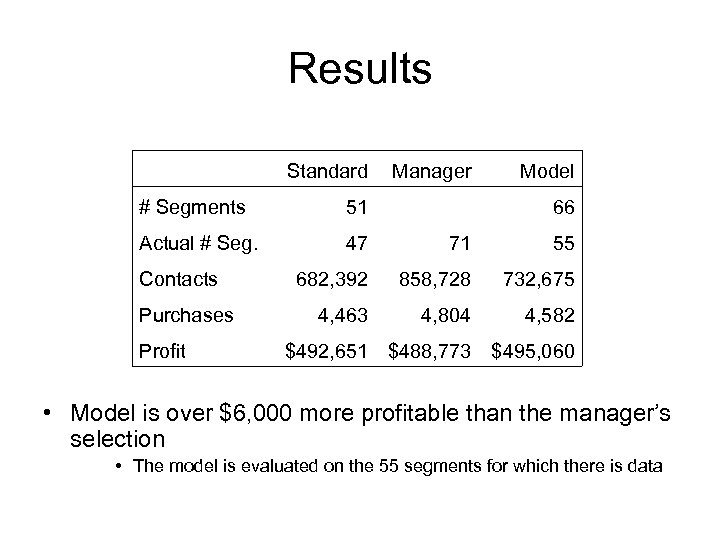
Results Standard Manager Model # Segments 51 Actual # Seg. 47 71 55 682, 392 858, 728 732, 675 4, 463 4, 804 4, 582 Contacts Purchases Profit 66 $492, 651 $488, 773 $495, 060 • Model is over $6, 000 more profitable than the manager’s selection • The model is evaluated on the 55 segments for which there is data

Concepts Introduced • Binary choice processes • Beta-Binomial model • Regression to the mean – How to use models to allow for this effect • Bayes theorem – Empirical Bayes methods • Application of EB to direct marketing campaigns

Types of Observed Variables • Have introduced three types of behavioural outcomes – Timing – “when? ” – Counting – “how many? ” – Choice – “whether/which? ” • These are widely encountered in a range of situations

Applications of Timing Models • Product trial • Repeat purchasing • Response times – Direct mail – Mail or e-mail survey responses • Customer retention or attrition • Other durations – Time spent on a web site – Job tenure for salespersons

Applications of Counting Models • • Number of advertising exposures Number of pages viewed per web session Salesperson productivity Sales concentration among customers – E. g. 80/20 rule • Number of each item bought, or number of distinct items, per shopping occasion • Number of trips – Shopping, bus or plane travel, park visits, fishing

Applications of Choice Models • Brand choice, e. g. – choice modeling questionnaire (exclusive choice) – scanner panel data (non-exclusive choice) • Media exposure • Binary variables – Response • Direct mail • Click-through for Web banner advertisements • Survey non-response (non-contacts, refusals) – Brand usage, awareness, image/associations

Combined Models • Two outcome variables – Counting + counting • Purchase - # of shopping trips & # of units bought per trip • Web site traffic - # of visits & # of pages viewed per visit – Counting and timing • Purchases – spacing of trips & # of items bought/trip • Web site - # of visits & duration of each visit – Counting and choice • # of visits & whether trip involved purchase • choice of brand & # of units purchased

Generalisations • If there are problems with model fit, we can use a different distribution or relax the usual assumptions – Non-exponential distribution for purchasing intervals • E. g. gamma distribution (Exp=Gamma(1, β)) • Implies non-Poisson distribution of counts – Non-gamma or non-beta heterogeneity • E. g. never try/buy group – Non-stationarity – latent traits may change over time • However the usual models appear quite robust to departures from the standard distributions and assumptions

Other Extensions • Introducing covariates • Finite mixture/latent class models • Hierarchical Bayes methods – These account properly for uncertainty at the population/market level