5e069707ac9288ec377e7408d9d0e79f.ppt
- Количество слайдов: 110

Probability Boot camp Joel Barajas October 13 th 2008
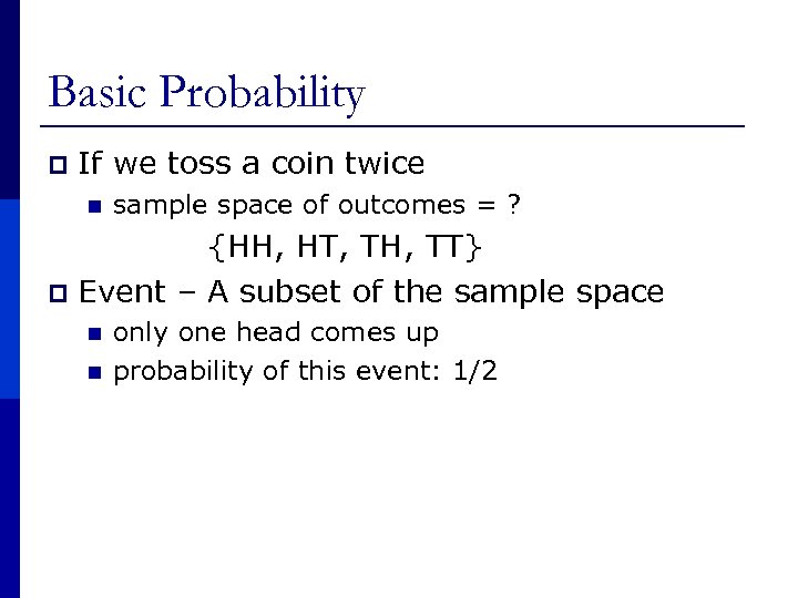
Basic Probability p If we toss a coin twice n sample space of outcomes = ? {HH, HT, TH, TT} p Event – A subset of the sample space n n only one head comes up probability of this event: 1/2
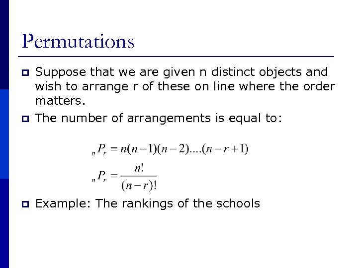
Permutations p Suppose that we are given n distinct objects and wish to arrange r of these on line where the order matters. The number of arrangements is equal to: p Example: The rankings of the schools p
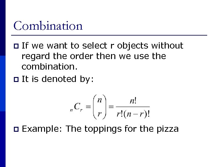
Combination If we want to select r objects without regard the order then we use the combination. p It is denoted by: p p Example: The toppings for the pizza
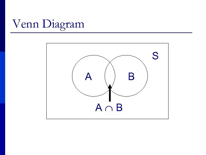
Venn Diagram S A B
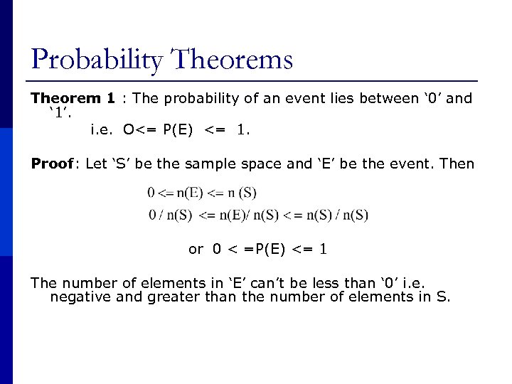
Probability Theorems Theorem 1 : The probability of an event lies between ‘ 0’ and ‘ 1’. i. e. O<= P(E) <= 1. Proof: Let ‘S’ be the sample space and ‘E’ be the event. Then or 0 < =P(E) <= 1 The number of elements in ‘E’ can’t be less than ‘ 0’ i. e. negative and greater than the number of elements in S.
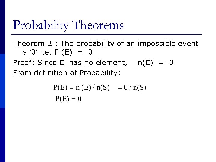
Probability Theorems Theorem 2 : The probability of an impossible event is ‘ 0’ i. e. P (E) = 0 Proof: Since E has no element, n(E) = 0 From definition of Probability:
Probability Theorems Theorem 3 : The probability of a sure event is 1. i. e. P(S) = 1. where ‘S’ is the sure event. Proof : In sure event n(E) = n(S) [ Since Number of elements in Event ‘E’ will be equal to the number of element in sample-space. ] By definition of Probability : P(S) = n (S)/ n (S) = 1 P(S) = 1
Probability Theorems Theorem 4: If two events ‘A’ and ‘B’ are such that A <=B, then P(A) < =P(B). Proof: n(A) < = n(B) or n(A) / N(S) < = n(B) / n(S) Then P(A) < =P(B) Since ‘A’ is the sub-set of ‘B”, so from set theory number of elements in ‘A’ can’t be more than number of element in ‘B’.
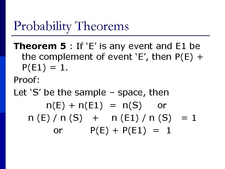
Probability Theorems Theorem 5 : If ‘E’ is any event and E 1 be the complement of event ‘E’, then P(E) + P(E 1) = 1. Proof: Let ‘S’ be the sample – space, then n(E) + n(E 1) = n(S) or n (E) / n (S) + n (E 1) / n (S) = 1 or P(E) + P(E 1) = 1
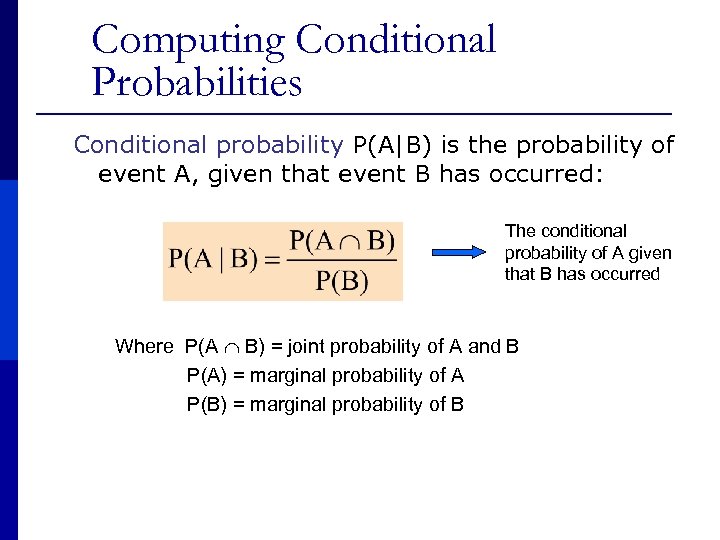
Computing Conditional Probabilities Conditional probability P(A|B) is the probability of event A, given that event B has occurred: The conditional probability of A given that B has occurred Where P(A B) = joint probability of A and B P(A) = marginal probability of A P(B) = marginal probability of B
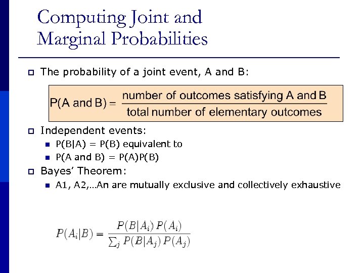
Computing Joint and Marginal Probabilities p The probability of a joint event, A and B: p Independent events: n n p P(B|A) = P(B) equivalent to P(A and B) = P(A)P(B) Bayes’ Theorem: n A 1, A 2, …An are mutually exclusive and collectively exhaustive
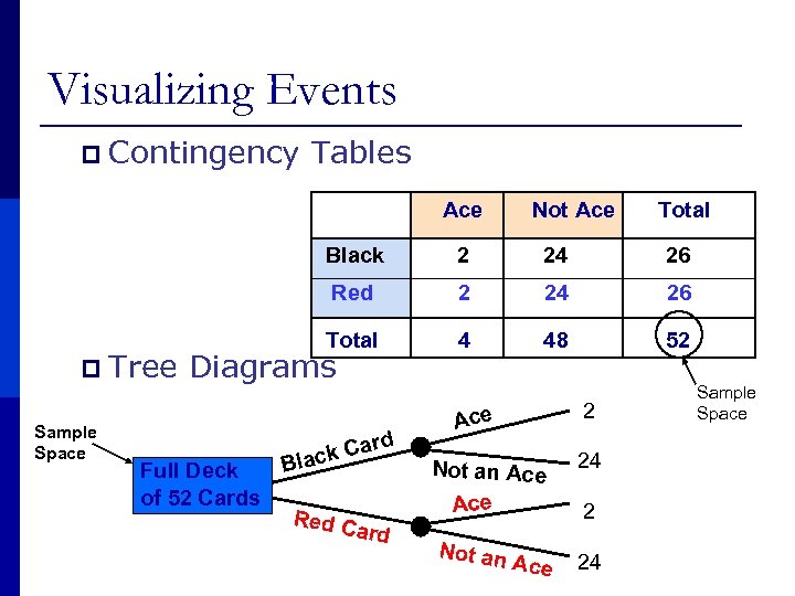
Visualizing Events p Contingency Tables Ace Not Ace Total Black 2 24 26 Red 2 24 26 Total 4 48 52 p Tree Diagrams Sample Space Full Deck of 52 Cards rd k Ca lac B Red C ard 2 Ace Not an 24 2 Ace 24 Sample Space
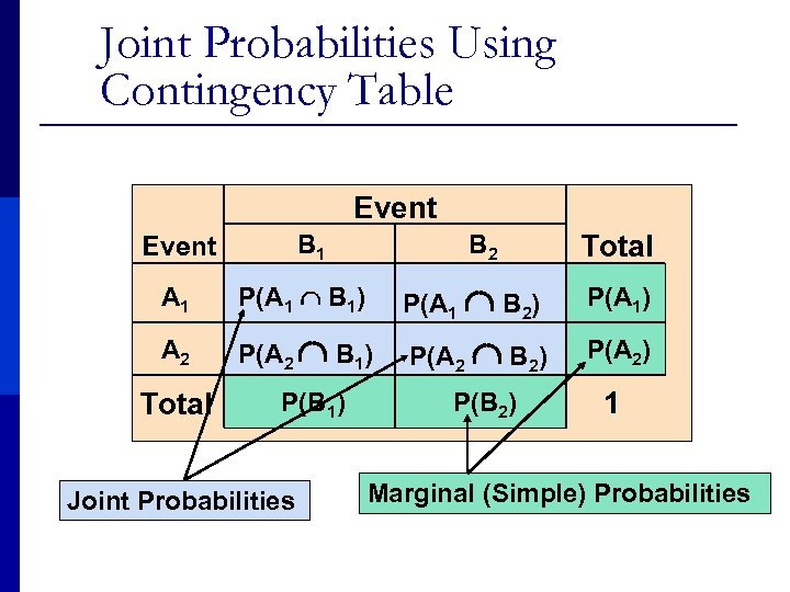
Joint Probabilities Using Contingency Table Event B 1 Event B 2 Total A 1 P(A 1 B 1) P(A 1 B 2) P(A 1) A 2 P(A 2 B 1) P(A 2 B 2) P(A 2) Total P(B 1) P(B 2) 1 Joint Probabilities Marginal (Simple) Probabilities
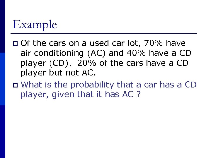
Example Of the cars on a used car lot, 70% have air conditioning (AC) and 40% have a CD player (CD). 20% of the cars have a CD player but not AC. p What is the probability that a car has a CD player, given that it has AC ? p
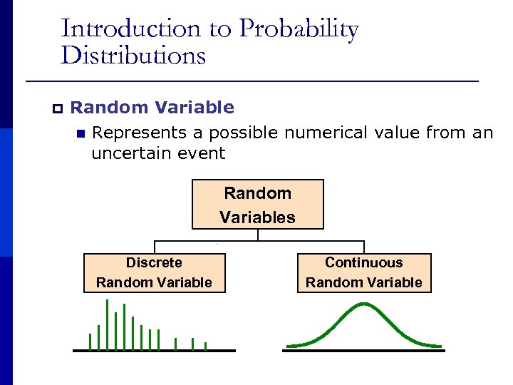
Introduction to Probability Distributions p Random Variable n Represents a possible numerical value from an uncertain event Random Variables Discrete Random Variable Continuous Random Variable
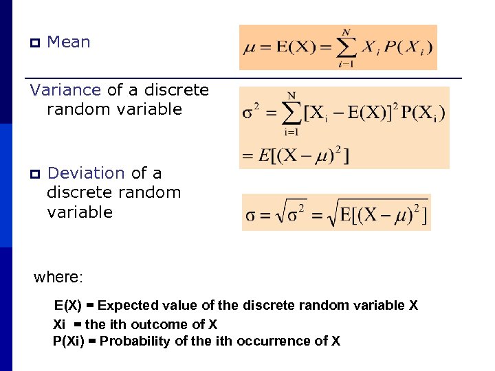
p Mean Variance of a discrete random variable p Deviation of a discrete random variable where: E(X) = Expected value of the discrete random variable X Xi = the ith outcome of X P(Xi) = Probability of the ith occurrence of X
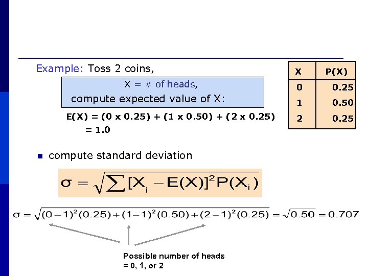
Example: Toss 2 coins, X = # of heads, compute expected value of X: E(X) = (0 x 0. 25) + (1 x 0. 50) + (2 x 0. 25) = 1. 0 n compute standard deviation Possible number of heads = 0, 1, or 2 X P(X) 0 0. 25 1 0. 50 2 0. 25
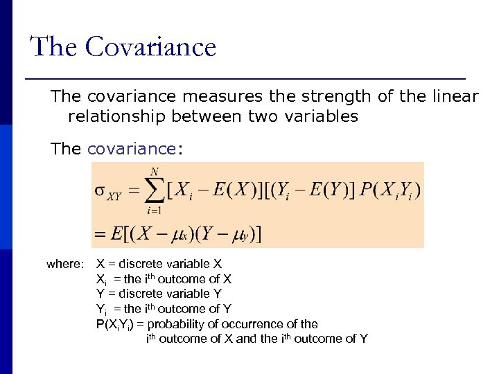
The Covariance The covariance measures the strength of the linear relationship between two variables The covariance: where: X = discrete variable X Xi = the ith outcome of X Y = discrete variable Y Yi = the ith outcome of Y P(Xi. Yi) = probability of occurrence of the ith outcome of X and the ith outcome of Y
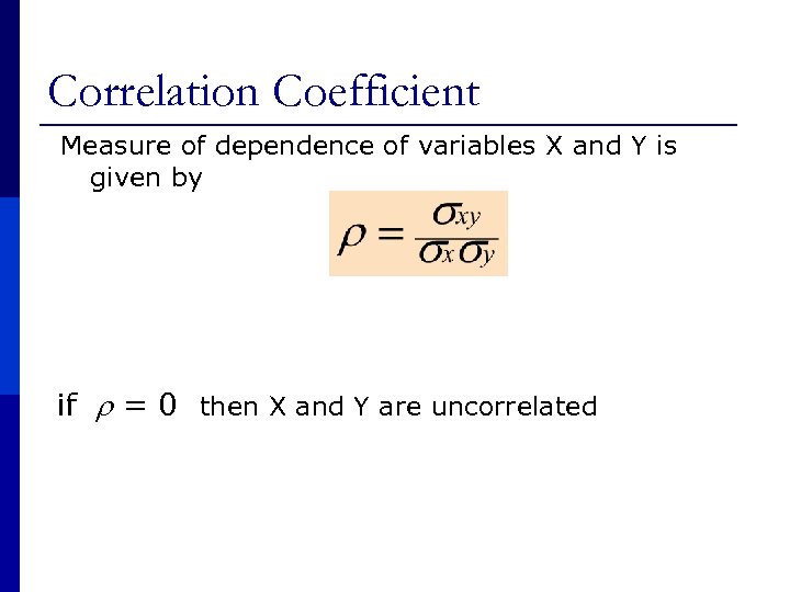
Correlation Coefficient Measure of dependence of variables X and Y is given by if = 0 then X and Y are uncorrelated
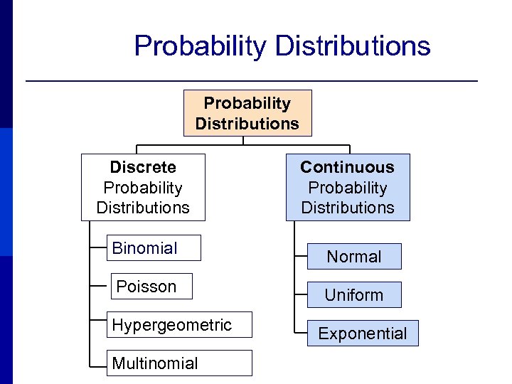
Probability Distributions Discrete Probability Distributions Continuous Probability Distributions Binomial Normal Poisson Uniform Hypergeometric Multinomial Exponential
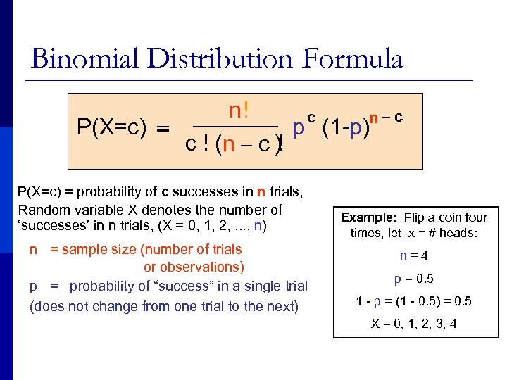
Binomial Distribution Formula n! c n c P(X=c) = p (1 -p) c ! (n - c )! P(X=c) = probability of c successes in n trials, Random variable X denotes the number of ‘successes’ in n trials, (X = 0, 1, 2, . . . , n) n = sample size (number of trials or observations) p = probability of “success” in a single trial (does not change from one trial to the next) Example: Flip a coin four times, let x = # heads: n=4 p = 0. 5 1 - p = (1 - 0. 5) = 0. 5 X = 0, 1, 2, 3, 4
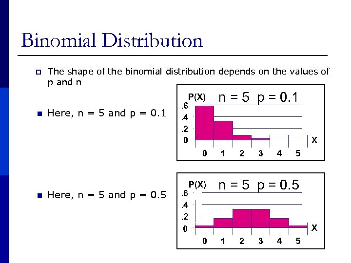
Binomial Distribution p The shape of the binomial distribution depends on the values of p and n Mean n Here, n = 5 and p = 0. 1 . 6. 4. 2 0 P(X) X 0 n Here, n = 5 and p = 0. 5 . 6. 4. 2 0 n = 5 p = 0. 1 P(X) 1 2 3 4 5 n = 5 p = 0. 5 X 0 1 2 3 4 5
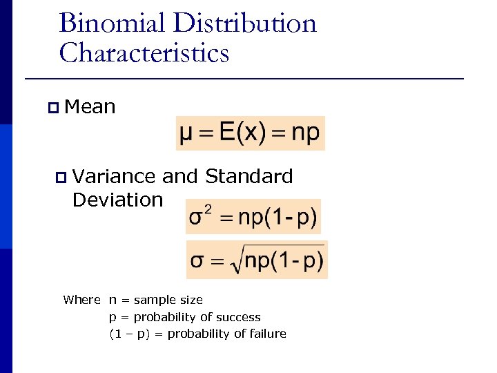
Binomial Distribution Characteristics p Mean p Variance and Standard Deviation Where n = sample size p = probability of success (1 – p) = probability of failure
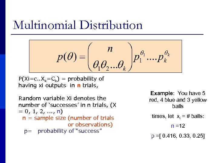
Multinomial Distribution P(Xi=c. . Xk=Ck) = probability of having xi outputs in n trials, Random variable Xi denotes the number of ‘successes’ in n trials, (X = 0, 1, 2, . . . , n) n = sample size (number of trials or observations) p= probability of “success” Example: You have 5 red, 4 blue and 3 yellow balls times, let xi = # balls: n =12 p =[ 0. 416, 0. 33, 0. 25]
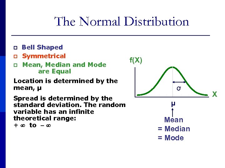
The Normal Distribution p ‘Bell p p Shaped’ Symmetrical Mean, Median and Mode are Equal f(X) Location is determined by the mean, μ Spread is determined by the standard deviation. The random variable has an infinite theoretical range: + to σ μ Mean = Median = Mode X
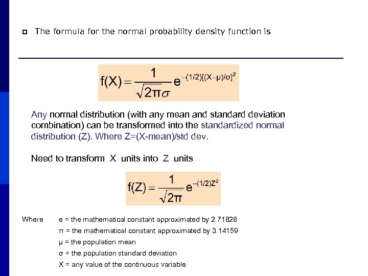
p The formula for the normal probability density function is Any normal distribution (with any mean and standard deviation combination) can be transformed into the standardized normal distribution (Z). Where Z=(X-mean)/std dev. Need to transform X units into Z units Where e = the mathematical constant approximated by 2. 71828 π = the mathematical constant approximated by 3. 14159 μ = the population mean σ = the population standard deviation X = any value of the continuous variable
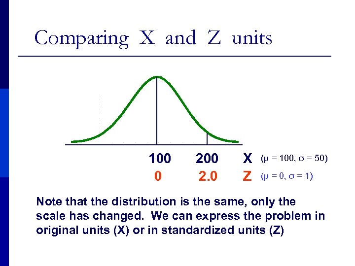
Comparing X and Z units 100 0 200 2. 0 X Z (μ = 100, σ = 50) (μ = 0, σ = 1) Note that the distribution is the same, only the scale has changed. We can express the problem in original units (X) or in standardized units (Z)
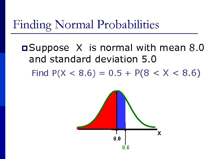
Finding Normal Probabilities p Suppose X is normal with mean 8. 0 and standard deviation 5. 0 Find P(X < 8. 6) = 0. 5 + P(8 < X < 8. 6) X 8. 0 8. 6
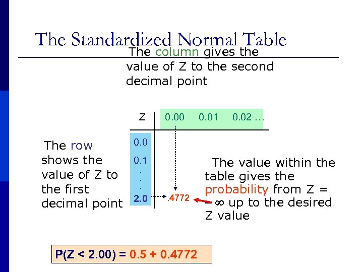
The Standardized Normal Table The column gives the value of Z to the second decimal point Z 0. 0 The row 0. 1 shows the value of Z to . . . the first decimal point 2. 0 0. 01 0. 02 … The value within the . 4772 2. 0 P(Z < 2. 00) = 0. 5 + 0. 4772 table gives the probability from Z = up to the desired Z value
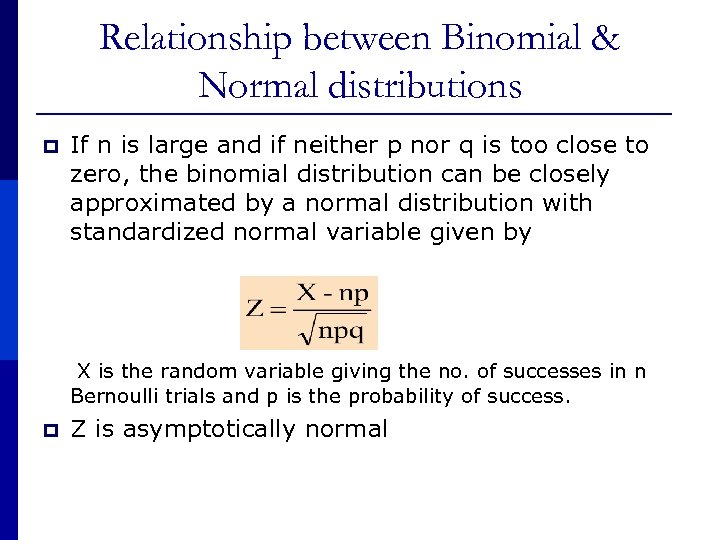
Relationship between Binomial & Normal distributions p If n is large and if neither p nor q is too close to zero, the binomial distribution can be closely approximated by a normal distribution with standardized normal variable given by X is the random variable giving the no. of successes in n Bernoulli trials and p is the probability of success. p Z is asymptotically normal
Normal Approximation to the Binomial Distribution p p p The binomial distribution is a discrete distribution, but the normal is continuous To use the normal to approximate the binomial, accuracy is improved if you use a correction for continuity adjustment Example: n X is discrete in a binomial distribution, so P(X = 4) can be approximated with a continuous normal distribution by finding P(3. 5 < X < 4. 5)
Normal Approximation to the Binomial Distribution p p p (continued) The closer p is to 0. 5, the better the normal approximation to the binomial The larger the sample size n, the better the normal approximation to the binomial General rule: n The normal distribution can be used to approximate the binomial distribution if np ≥ 5 and n(1 – p) ≥ 5
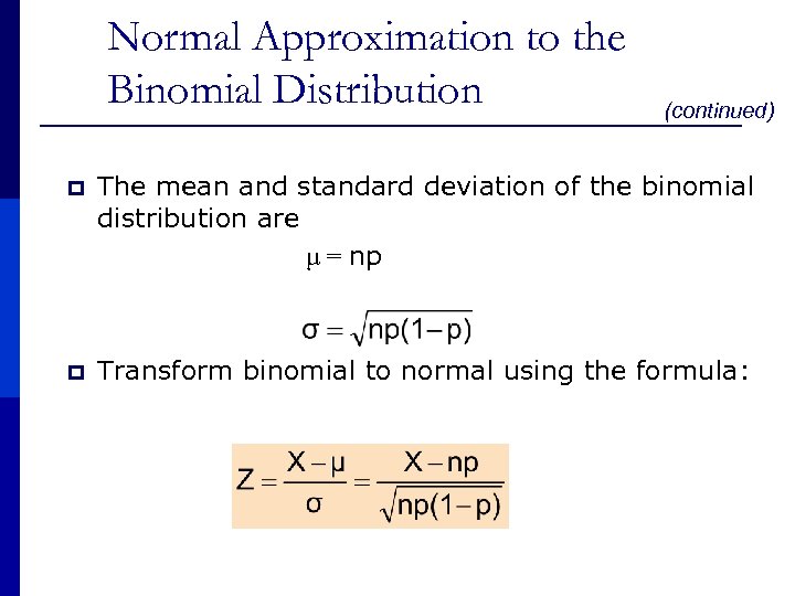
Normal Approximation to the Binomial Distribution p (continued) The mean and standard deviation of the binomial distribution are μ = np p Transform binomial to normal using the formula:
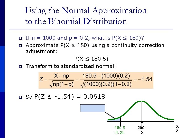
Using the Normal Approximation to the Binomial Distribution p If n = 1000 and p = 0. 2, what is P(X ≤ 180)? Approximate P(X ≤ 180) using a continuity correction adjustment: P(X ≤ 180. 5) Transform to standardized normal: p So P(Z ≤ -1. 54) = 0. 0618 p p 180. 5 -1. 54 200 0 X Z
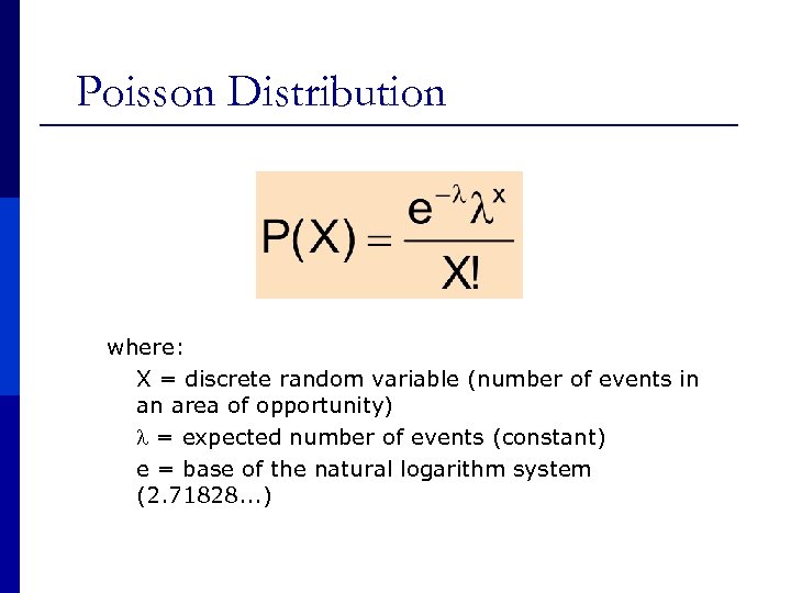
Poisson Distribution where: X = discrete random variable (number of events in an area of opportunity) = expected number of events (constant) e = base of the natural logarithm system (2. 71828. . . )
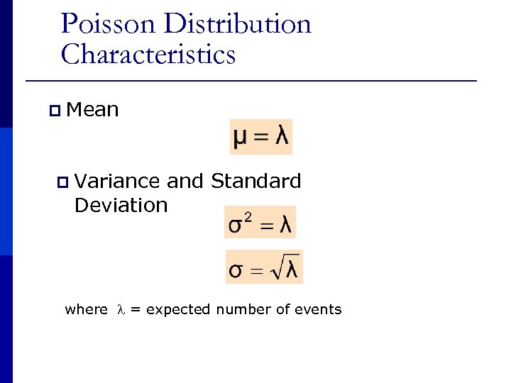
Poisson Distribution Characteristics p Mean p Variance and Standard Deviation where = expected number of events
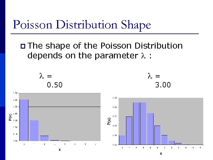
Poisson Distribution Shape p The shape of the Poisson Distribution depends on the parameter : = 0. 50 = 3. 00
Relationship between Poisson & Normal distributions p In a Binomial Distribution if n is large and p is small ( probability of success ) then it approximates to Poisson Distribution with = np.
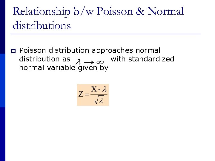
Relationship b/w Poisson & Normal distributions p Poisson distribution approaches normal distribution as with standardized normal variable given by
Are there any other distributions besides binomial and Poisson that have the normal distribution as the limiting case?
The Uniform Distribution p The uniform distribution is a probability distribution that has equal probabilities for all possible outcomes of the random variable p Also called a rectangular distribution
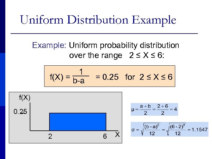
Uniform Distribution Example: Uniform probability distribution over the range 2 ≤ X ≤ 6: 1 f(X) = b-a = 0. 25 for 2 ≤ X ≤ 6 f(X) 0. 25 2 6 X
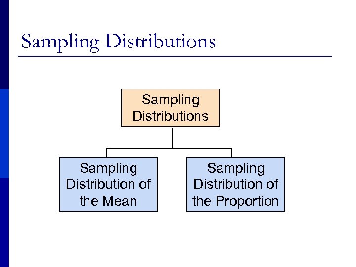
Sampling Distributions Sampling Distribution of the Mean Sampling Distribution of the Proportion
Sampling Distributions p A sampling distribution is a distribution of all of the possible values of a statistic for a given size sample selected from a population
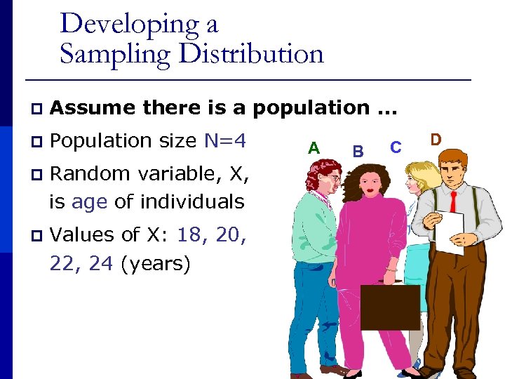
Developing a Sampling Distribution p Assume there is a population … p Population size N=4 p Random variable, X, is age of individuals p Values of X: 18, 20, 22, 24 (years) A B C D
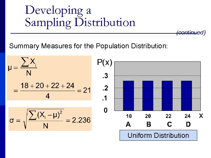
Developing a Sampling Distribution (continued) Summary Measures for the Population Distribution: P(x). 3. 2. 1 0 18 20 22 24 A B C D Uniform Distribution x
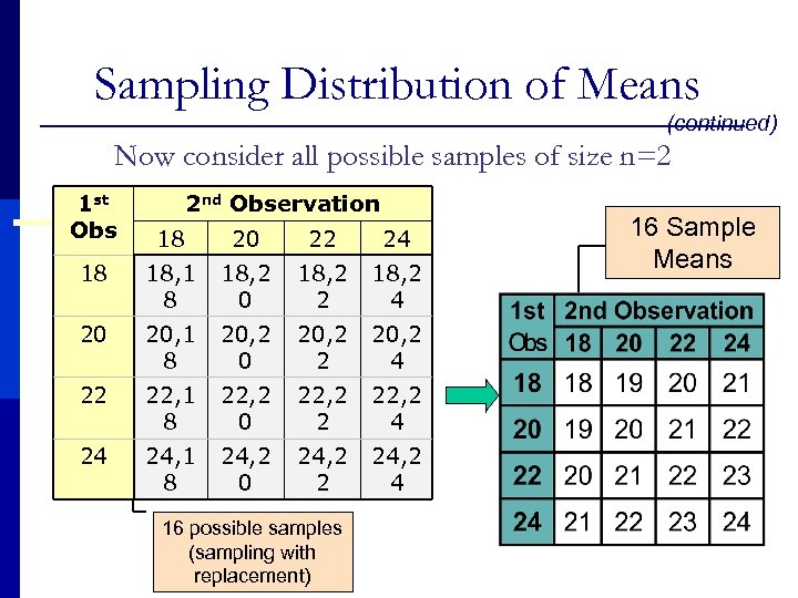
Sampling Distribution of Means (continued) Now consider all possible samples of size n=2 1 st Obs 2 nd Observation 18 20 22 24 18 18, 1 8 18, 2 0 18, 2 2 18, 2 4 20 20, 1 8 20, 2 0 20, 2 2 20, 2 4 22 22, 1 8 22, 2 0 22, 2 2 22, 2 4 24 24, 1 8 24, 2 0 24, 2 2 24, 2 4 16 possible samples (sampling with replacement) 16 Sample Means
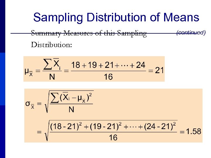
Sampling Distribution of Means Summary Measures of this Sampling Distribution: (continued)
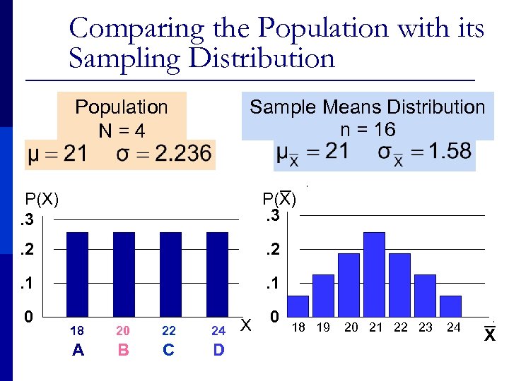
Comparing the Population with its Sampling Distribution Population N=4 Sample Means Distribution n = 16 _ P(X). 3 . 2 . 1 0 18 20 22 24 A B C D X 0 18 19 20 21 22 23 24 _ X
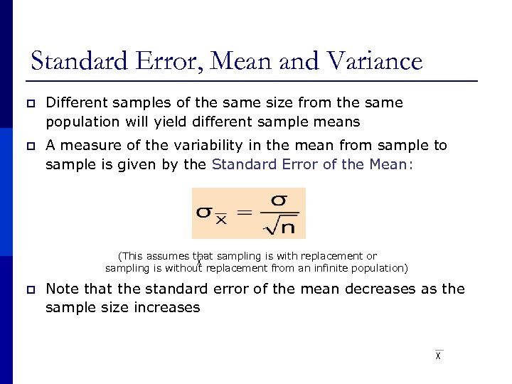
Standard Error, Mean and Variance p Different samples of the same size from the same population will yield different sample means p A measure of the variability in the mean from sample to sample is given by the Standard Error of the Mean: (This assumes that sampling is with replacement or sampling is without replacement from an infinite population) p Note that the standard error of the mean decreases as the sample size increases
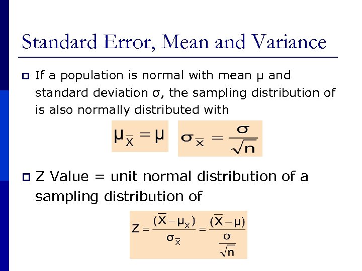
Standard Error, Mean and Variance p If a population is normal with mean μ and standard deviation σ, the sampling distribution of is also normally distributed with p Z Value = unit normal distribution of a sampling distribution of
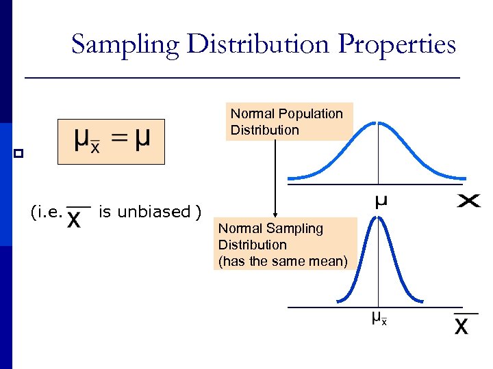
Sampling Distribution Properties Normal Population Distribution p (i. e. is unbiased ) Normal Sampling Distribution (has the same mean)
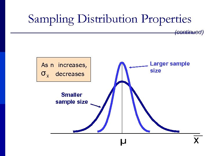
Sampling Distribution Properties (continued) As n increases, decreases Smaller sample size Larger sample size
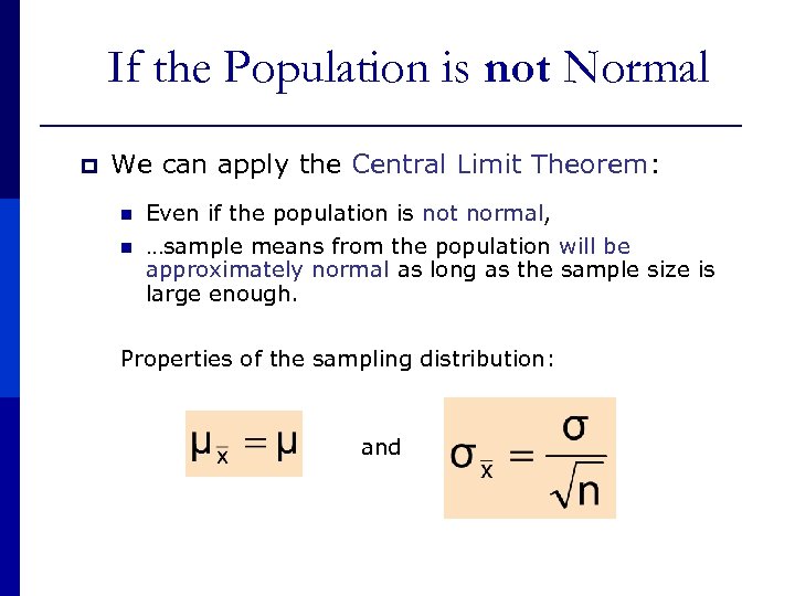
If the Population is not Normal p We can apply the Central Limit Theorem: n n Even if the population is not normal, …sample means from the population will be approximately normal as long as the sample size is large enough. Properties of the sampling distribution: and
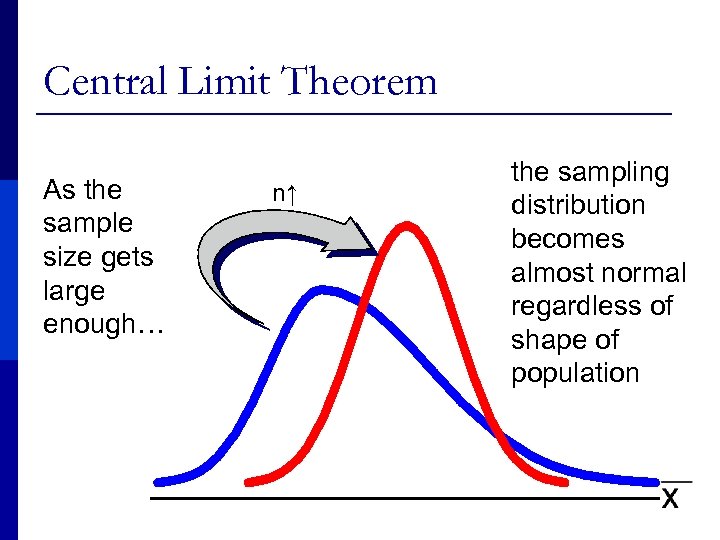
Central Limit Theorem As the sample size gets large enough… n↑ the sampling distribution becomes almost normal regardless of shape of population
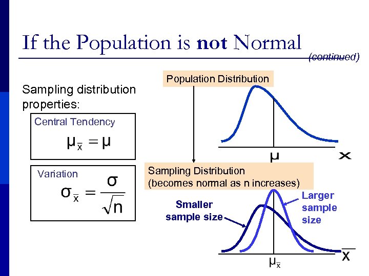
If the Population is not Normal Sampling distribution properties: (continued) Population Distribution Central Tendency Variation Sampling Distribution (becomes normal as n increases) Smaller sample size Larger sample size
How Large is Large Enough? p For most distributions, n > 30 will give a sampling distribution that is nearly normal p For fairly symmetric distributions, n > 15 p For normal population distributions, the sampling distribution of the mean is always normally distributed
Example p Suppose a population has mean μ = 8 and standard deviation σ = 3. Suppose a random sample of size n = 36 is selected. p What is the probability that the sample mean is between 7. 8 and 8. 2?
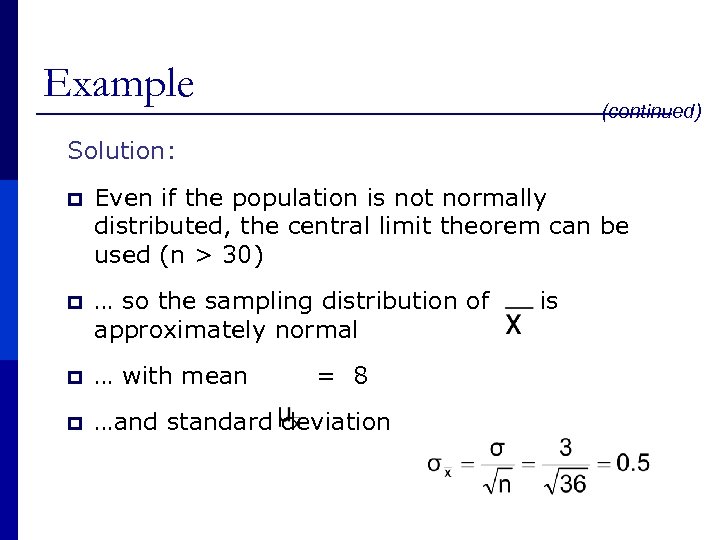
Example (continued) Solution: p Even if the population is not normally distributed, the central limit theorem can be used (n > 30) p … so the sampling distribution of is approximately normal p … with mean = 8 p …and standard deviation
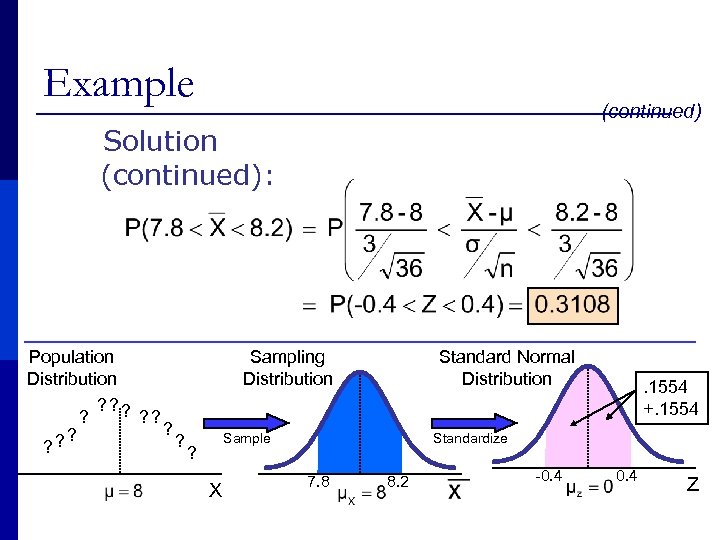
Example (continued) Solution (continued): Population Distribution ? ? ? Sampling Distribution Standard Normal Distribution Sample ? X . 1554 +. 1554 Standardize 7. 8 8. 2 -0. 4 Z
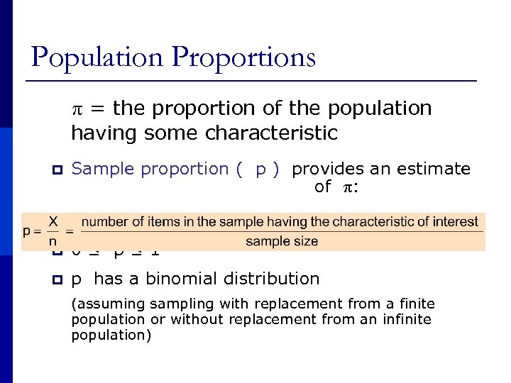
Population Proportions π = the proportion of the population having some characteristic Sample proportion ( p ) provides an estimate of π: p p 0 ≤ p ≤ 1 p p has a binomial distribution (assuming sampling with replacement from a finite population or without replacement from an infinite population)
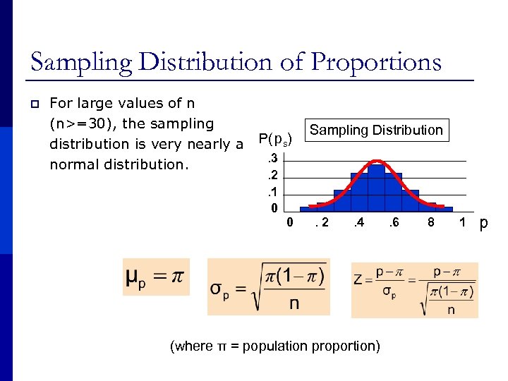
Sampling Distribution of Proportions p For large values of n (n>=30), the sampling distribution is very nearly a P( ps). 3 normal distribution. . 2. 1 0 0 Sampling Distribution . 2 . 4 (where π = population proportion) . 6 8 1 p
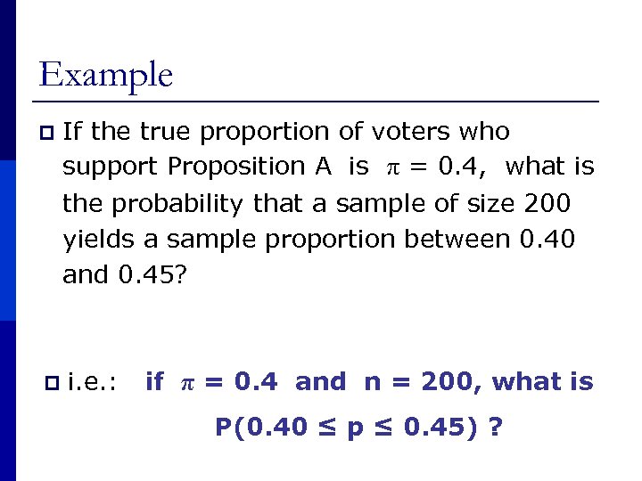
Example p If the true proportion of voters who support Proposition A is π = 0. 4, what is the probability that a sample of size 200 yields a sample proportion between 0. 40 and 0. 45? p i. e. : if π = 0. 4 and n = 200, what is P(0. 40 ≤ p ≤ 0. 45) ?
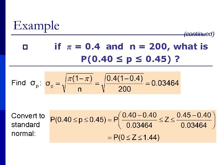
Example p Find (continued) if π = 0. 4 and n = 200, what is P(0. 40 ≤ p ≤ 0. 45) ? : Convert to standard normal:
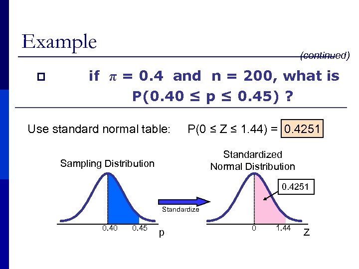
Example p (continued) if π = 0. 4 and n = 200, what is P(0. 40 ≤ p ≤ 0. 45) ? Use standard normal table: P(0 ≤ Z ≤ 1. 44) = 0. 4251 Standardized Normal Distribution Sampling Distribution 0. 4251 Standardize 0. 40 0. 45 p 0 1. 44 Z
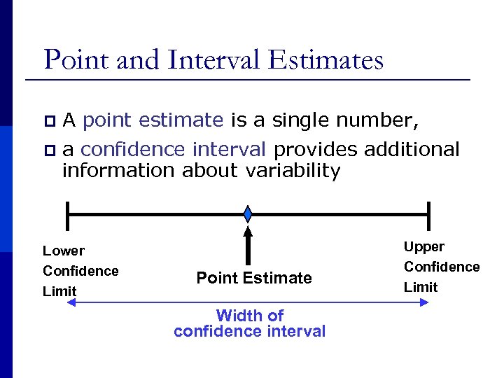
Point and Interval Estimates p A point estimate is a single number, p a confidence interval provides additional information about variability Lower Confidence Limit Point Estimate Width of confidence interval Upper Confidence Limit
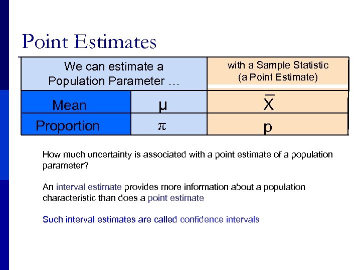
Point Estimates We can estimate a Population Parameter … Mean Proportion with a Sample Statistic (a Point Estimate) μ π X p How much uncertainty is associated with a point estimate of a population parameter? An interval estimate provides more information about a population characteristic than does a point estimate Such interval estimates are called confidence intervals
Confidence Interval Estimate p An interval gives a range of values: n Takes into consideration variation in sample statistics from sample to sample n Based on observations from 1 sample n Gives information about closeness to unknown population parameters n Stated in terms of level of confidence p Can never be 100% confident
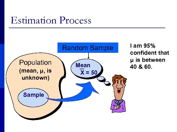
Estimation Process Random Sample Population (mean, μ, is unknown) Sample Mean X = 50 I am 95% confident that μ is between 40 & 60.
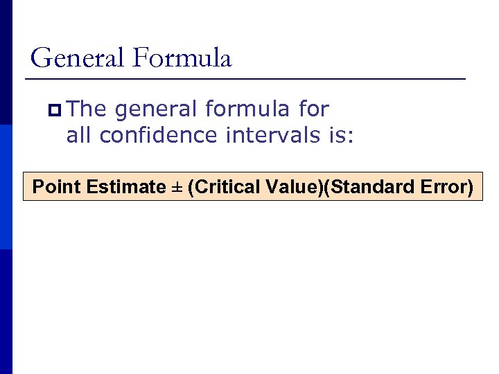
General Formula p The general formula for all confidence intervals is: Point Estimate ± (Critical Value)(Standard Error)
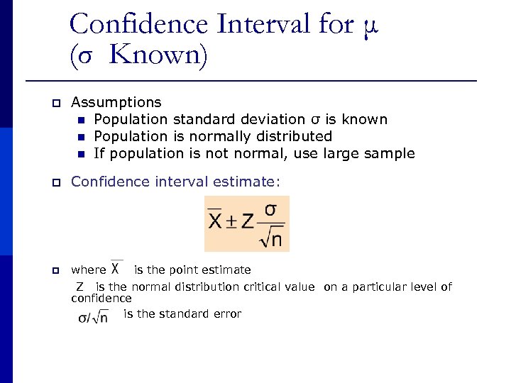
Confidence Interval for μ (σ Known) p Assumptions n Population standard deviation σ is known n Population is normally distributed n If population is not normal, use large sample p Confidence interval estimate: p where is the point estimate Z is the normal distribution critical value on a particular level of confidence is the standard error
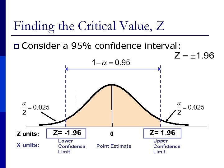
Finding the Critical Value, Z p Consider a 95% confidence interval: Z units: X units: Z= -1. 96 Lower Confidence Limit 0 Point Estimate Z= 1. 96 Upper Confidence Limit
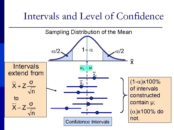
Intervals and Level of Confidence Sampling Distribution of the Mean x Intervals extend from x 1 x 2 to Confidence Intervals (1 - )x 100% of intervals constructed contain μ; ( )x 100% do not.
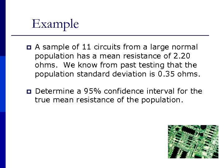
Example p A sample of 11 circuits from a large normal population has a mean resistance of 2. 20 ohms. We know from past testing that the population standard deviation is 0. 35 ohms. p Determine a 95% confidence interval for the true mean resistance of the population.
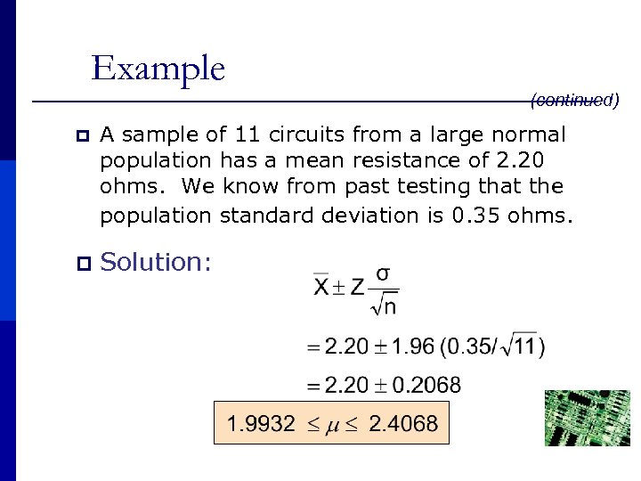
Example (continued) p A sample of 11 circuits from a large normal population has a mean resistance of 2. 20 ohms. We know from past testing that the population standard deviation is 0. 35 ohms. p Solution:
Interpretation p We are 95% confident that the true mean resistance is between 1. 9932 and 2. 4068 ohms p Although the true mean may or may not be in this interval, 95% of intervals formed in this manner will contain the true mean
Confidence Interval for μ (σ Unknown) p If the population standard deviation σ is unknown, we can substitute the sample standard deviation, S p This introduces extra uncertainty, since S is variable from sample to sample p So we use the t distribution instead of the normal distribution
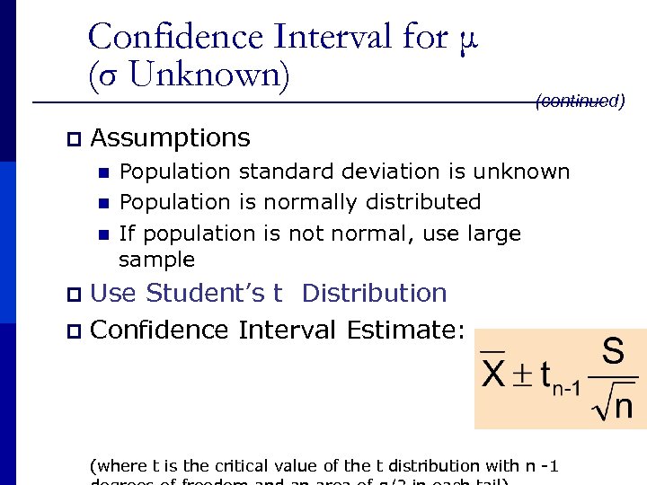
Confidence Interval for μ (σ Unknown) p (continued) Assumptions n n n Population standard deviation is unknown Population is normally distributed If population is not normal, use large sample Use Student’s t Distribution p Confidence Interval Estimate: p (where t is the critical value of the t distribution with n -1
Student’s t Distribution p The t is a family of distributions p The t value depends on degrees of freedom (d. f. ) n Number of observations that are free to vary after sample mean has been calculated d. f. = n - 1
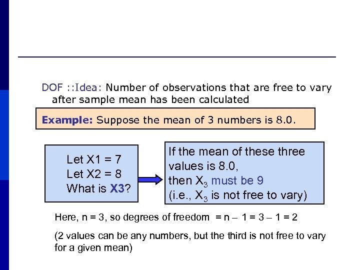
DOF : : Idea: Number of observations that are free to vary after sample mean has been calculated Example: Suppose the mean of 3 numbers is 8. 0. Let X 1 = 7 Let X 2 = 8 What is X 3? If the mean of these three values is 8. 0, then X 3 must be 9 (i. e. , X 3 is not free to vary) Here, n = 3, so degrees of freedom = n – 1 = 3 – 1 = 2 (2 values can be any numbers, but the third is not free to vary for a given mean)
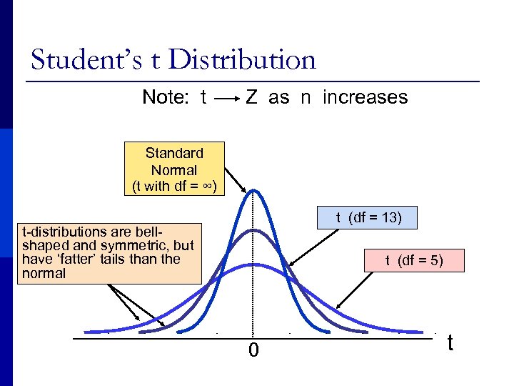
Student’s t Distribution Note: t Z as n increases Standard Normal (t with df = ∞) t (df = 13) t-distributions are bellshaped and symmetric, but have ‘fatter’ tails than the normal t (df = 5) 0 t
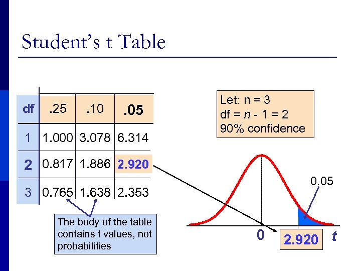
Student’s t Table df . 25 . 10 . 05 1 1. 000 3. 078 6. 314 Let: n = 3 df = n - 1 = 2 90% confidence 2 0. 817 1. 886 2. 920 0. 05 3 0. 765 1. 638 2. 353 The body of the table contains t values, not probabilities 0 2. 920 t
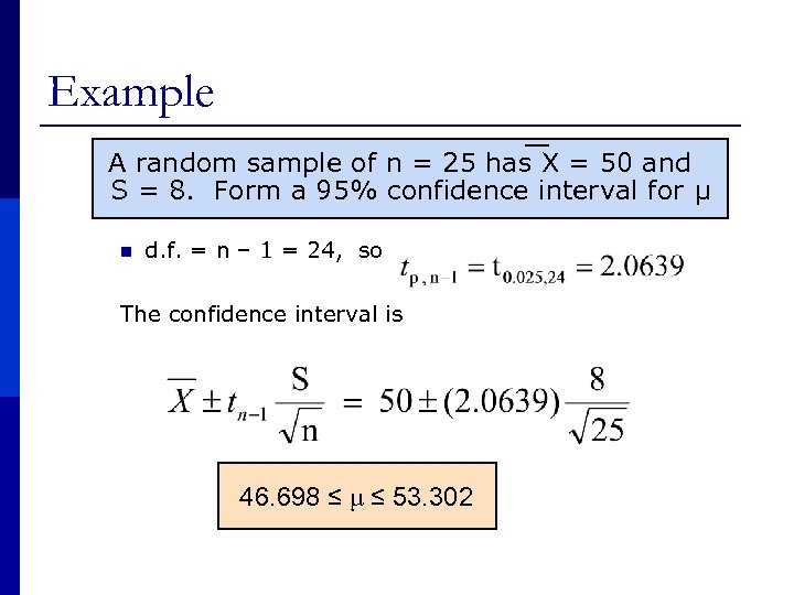
Example A random sample of n = 25 has X = 50 and S = 8. Form a 95% confidence interval for μ n d. f. = n – 1 = 24, so The confidence interval is 46. 698 ≤ μ ≤ 53. 302
What is a Hypothesis? p A hypothesis is a claim (assumption) about a population parameter: n population mean Example: The mean monthly cell phone bill of this city is μ = $42 n population proportion Example: The proportion of adults in this city with cell phones is π = 0. 68
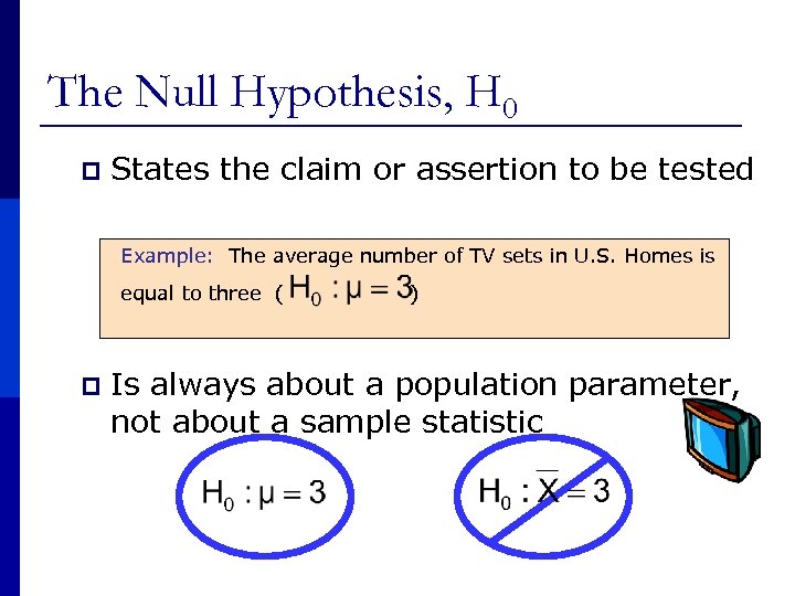
The Null Hypothesis, H 0 p States the claim or assertion to be tested Example: The average number of TV sets in U. S. Homes is equal to three ( ) p Is always about a population parameter, not about a sample statistic
The Null Hypothesis, H 0 (continued) p p p Begin with the assumption that the null hypothesis is true Always contains “=” , “≤” or “ ” sign May or may not be rejected
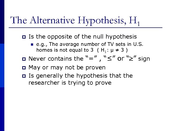
The Alternative Hypothesis, H 1 p Is the opposite of the null hypothesis n p p p e. g. , The average number of TV sets in U. S. homes is not equal to 3 ( H 1: μ ≠ 3 ) Never contains the “=” , “≤” or “ ” sign May or may not be proven Is generally the hypothesis that the researcher is trying to prove
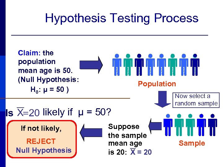
Hypothesis Testing Process Claim: the population mean age is 50. (Null Hypothesis: H 0: μ = 50 ) Population Is X= 20 likely if μ = 50? If not likely, REJECT Null Hypothesis Suppose the sample mean age is 20: X = 20 Now select a random sample Sample
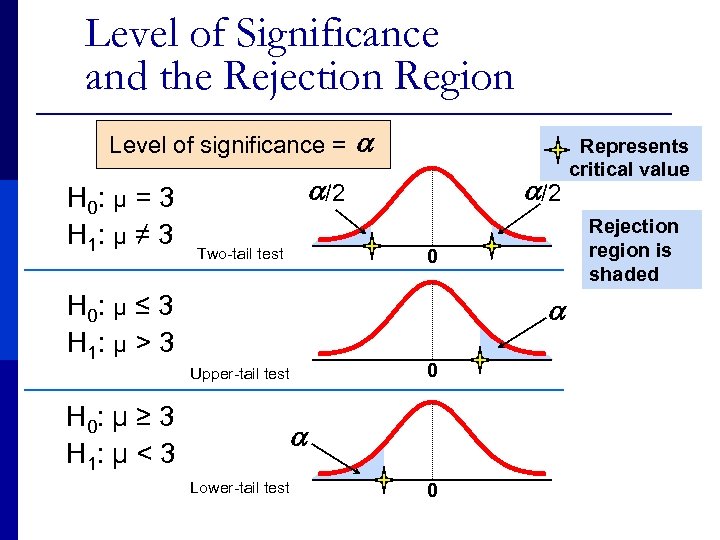
Level of Significance and the Rejection Region Level of significance = H 0: μ = 3 H 1: μ ≠ 3 /2 Two-tail test /2 Upper-tail test 0 Lower-tail test 0 Represents critical value Rejection region is shaded 0 H 0: μ ≤ 3 H 1: μ > 3 H 0: μ ≥ 3 H 1: μ < 3
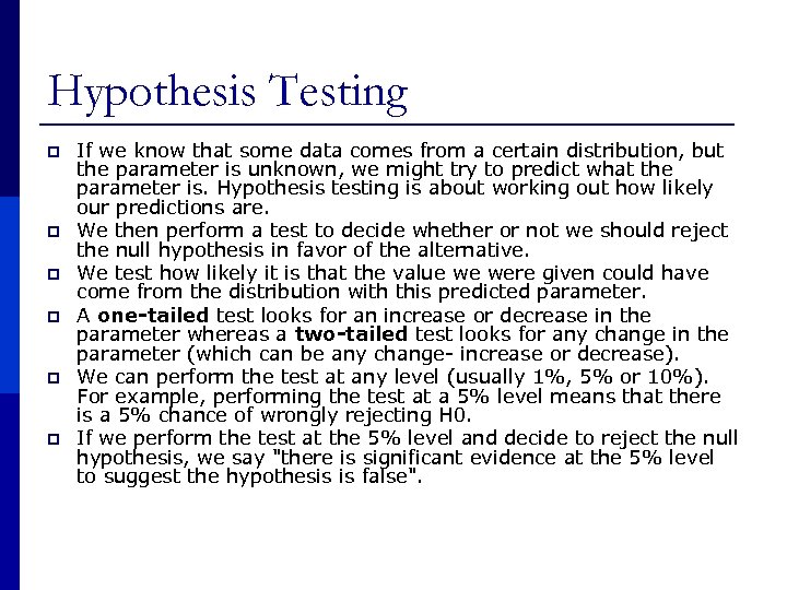
Hypothesis Testing p p p If we know that some data comes from a certain distribution, but the parameter is unknown, we might try to predict what the parameter is. Hypothesis testing is about working out how likely our predictions are. We then perform a test to decide whether or not we should reject the null hypothesis in favor of the alternative. We test how likely it is that the value we were given could have come from the distribution with this predicted parameter. A one-tailed test looks for an increase or decrease in the parameter whereas a two-tailed test looks for any change in the parameter (which can be any change- increase or decrease). We can perform the test at any level (usually 1%, 5% or 10%). For example, performing the test at a 5% level means that there is a 5% chance of wrongly rejecting H 0. If we perform the test at the 5% level and decide to reject the null hypothesis, we say "there is significant evidence at the 5% level to suggest the hypothesis is false".
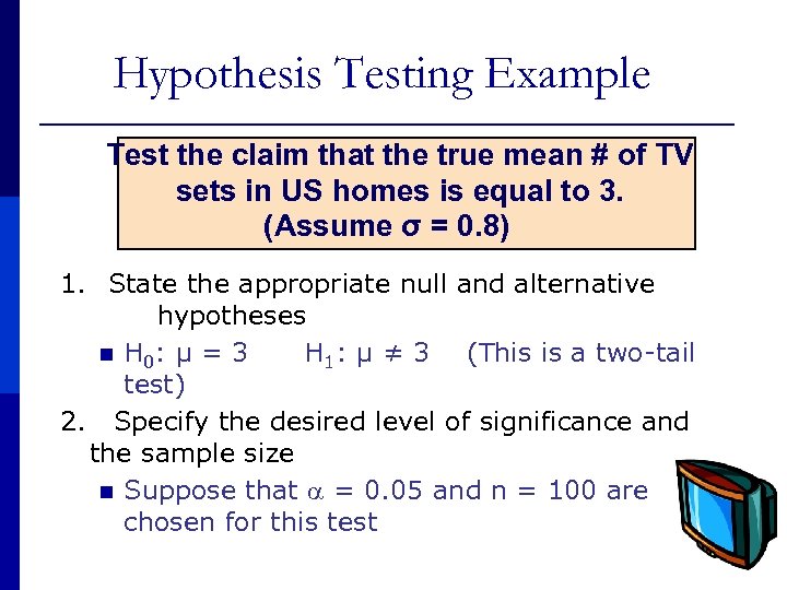
Hypothesis Testing Example Test the claim that the true mean # of TV sets in US homes is equal to 3. (Assume σ = 0. 8) 1. State the appropriate null and alternative hypotheses n H 0: μ = 3 H 1: μ ≠ 3 (This is a two-tail test) 2. Specify the desired level of significance and the sample size n Suppose that = 0. 05 and n = 100 are chosen for this test
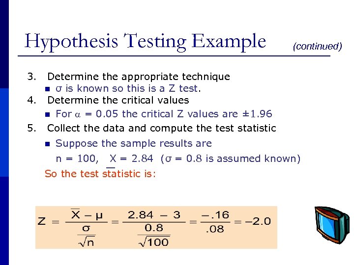
Hypothesis Testing Example (continued) 3. Determine the appropriate technique n σ is known so this is a Z test. 4. Determine the critical values n For = 0. 05 the critical Z values are ± 1. 96 5. Collect the data and compute the test statistic n Suppose the sample results are n = 100, X = 2. 84 (σ = 0. 8 is assumed known) So the test statistic is:
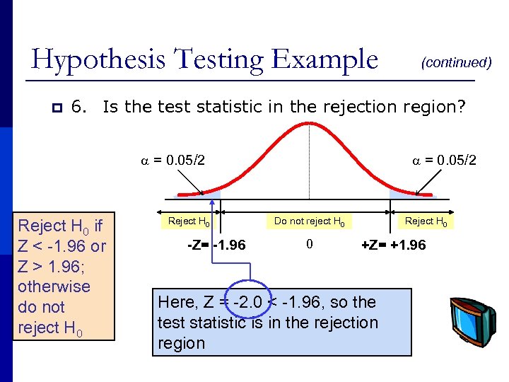
Hypothesis Testing Example p (continued) 6. Is the test statistic in the rejection region? = 0. 05/2 Reject H 0 if Z < -1. 96 or Z > 1. 96; otherwise do not reject H 0 Reject H 0 -Z= -1. 96 = 0. 05/2 Do not reject H 0 0 Reject H 0 +Z= +1. 96 Here, Z = -2. 0 < -1. 96, so the test statistic is in the rejection region
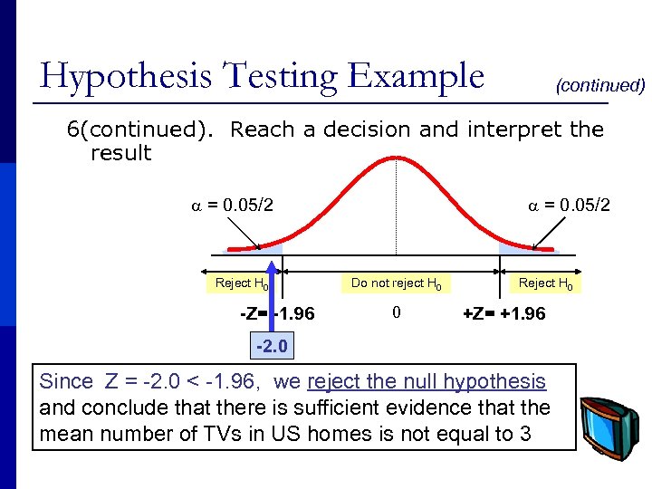
Hypothesis Testing Example (continued) 6(continued). Reach a decision and interpret the result = 0. 05/2 Reject H 0 -Z= -1. 96 = 0. 05/2 Do not reject H 0 0 Reject H 0 +Z= +1. 96 -2. 0 Since Z = -2. 0 < -1. 96, we reject the null hypothesis and conclude that there is sufficient evidence that the mean number of TVs in US homes is not equal to 3
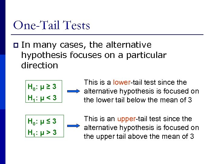
One-Tail Tests p In many cases, the alternative hypothesis focuses on a particular direction H 0: μ ≥ 3 H 1: μ < 3 H 0: μ ≤ 3 H 1: μ > 3 This is a lower-tail test since the alternative hypothesis is focused on the lower tail below the mean of 3 This is an upper-tail test since the alternative hypothesis is focused on the upper tail above the mean of 3
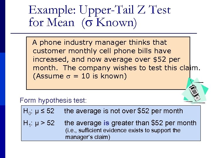
Example: Upper-Tail Z Test for Mean ( Known) A phone industry manager thinks that customer monthly cell phone bills have increased, and now average over $52 per month. The company wishes to test this claim. (Assume = 10 is known) Form hypothesis test: H 0: μ ≤ 52 the average is not over $52 per month H 1: μ > 52 the average is greater than $52 per month (i. e. , sufficient evidence exists to support the manager’s claim)
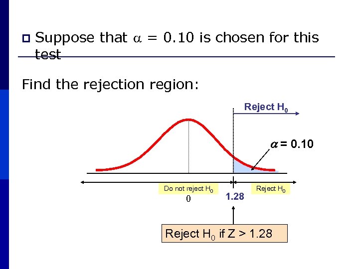
p Suppose that = 0. 10 is chosen for this test Find the rejection region: Reject H 0 = 0. 10 Do not reject H 0 0 1. 28 Reject H 0 if Z > 1. 28
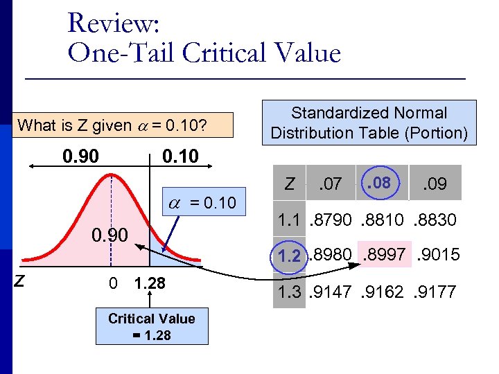
Review: One-Tail Critical Value What is Z given a = 0. 10? 0. 90 0. 10 a = 0. 10 0. 90 z Standardized Normal Distribution Table (Portion) 0 1. 28 Critical Value = 1. 28 Z . 07 . 08 . 09 1. 1. 8790. 8810. 8830 1. 2. 8980. 8997. 9015 1. 3. 9147. 9162. 9177
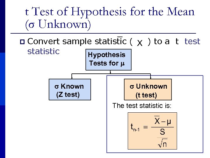
t Test of Hypothesis for the Mean (σ Unknown) p Convert sample statistic ( ) to a t test X statistic Hypothesis Tests for Known σ Known (Z test) Unknown σ Unknown (t test) The test statistic is:
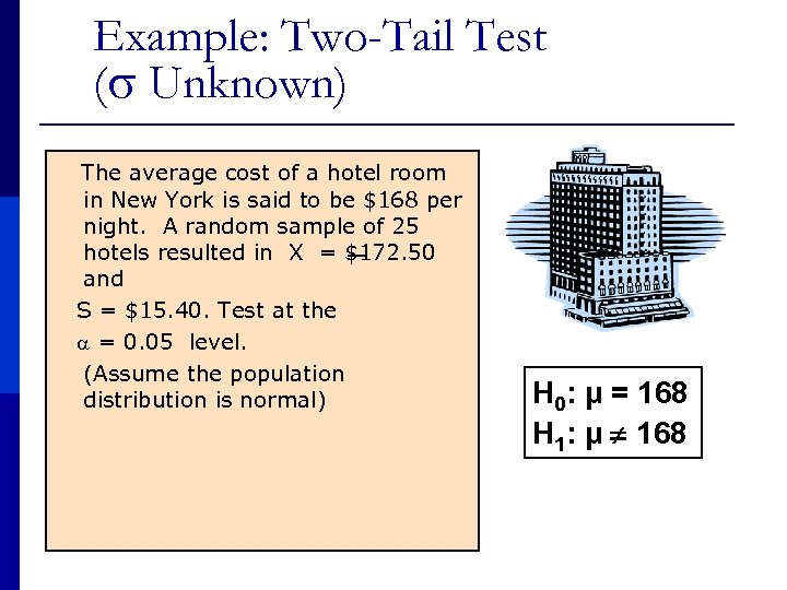
Example: Two-Tail Test ( Unknown) The average cost of a hotel room in New York is said to be $168 per night. A random sample of 25 hotels resulted in X = $172. 50 and S = $15. 40. Test at the = 0. 05 level. (Assume the population distribution is normal) H 0: μ = 168 H 1: μ ¹ 168
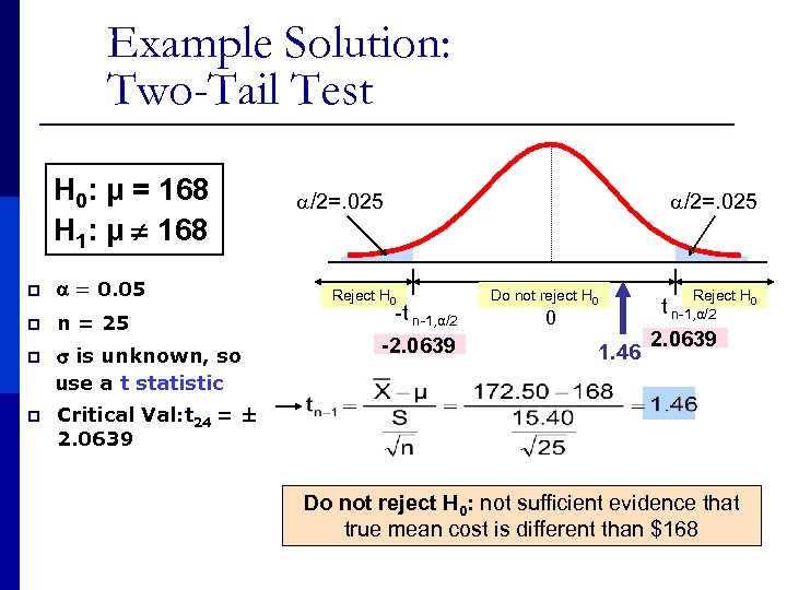
Example Solution: Two-Tail Test H 0: μ = 168 H 1: μ ¹ 168 p = 0. 05 p n = 25 p is unknown, so use a t statistic p /2=. 025 Critical Val: t 24 = ± 2. 0639 Reject H 0 -t n-1, α/2 -2. 0639 Do not reject H 0 0 1. 46 Reject H 0 t n-1, α/2 2. 0639 Do not reject H 0: not sufficient evidence that true mean cost is different than $168
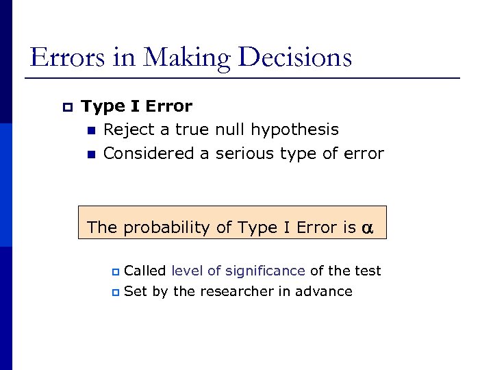
Errors in Making Decisions p Type I Error n Reject a true null hypothesis n Considered a serious type of error The probability of Type I Error is p Called level of significance of the test p Set by the researcher in advance
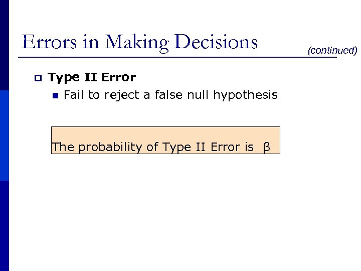
Errors in Making Decisions p Type II Error n Fail to reject a false null hypothesis The probability of Type II Error is β (continued)
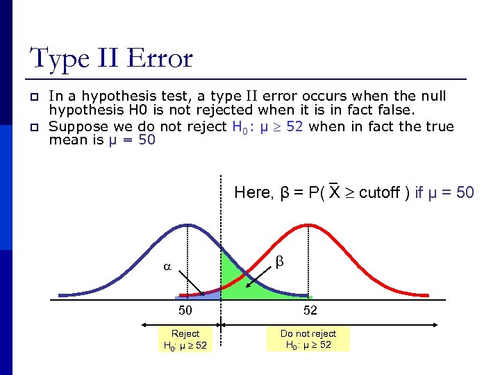
Type II Error p p In a hypothesis test, a type II error occurs when the null hypothesis H 0 is not rejected when it is in fact false. Suppose we do not reject H 0: μ 52 when in fact the true mean is μ = 50 Here, β = P( X cutoff ) if μ = 50 β 50 52 Reject H 0: μ 52 Do not reject H 0 : μ 52
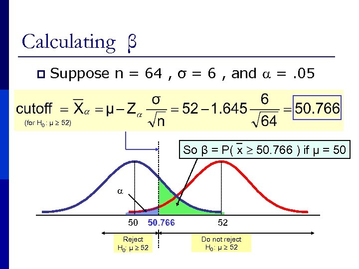
Calculating β p Suppose n = 64 , σ = 6 , and =. 05 (for H 0 : μ 52) So β = P( x 50. 766 ) if μ = 50 50. 766 Reject H 0: μ 52 52 Do not reject H 0 : μ 52
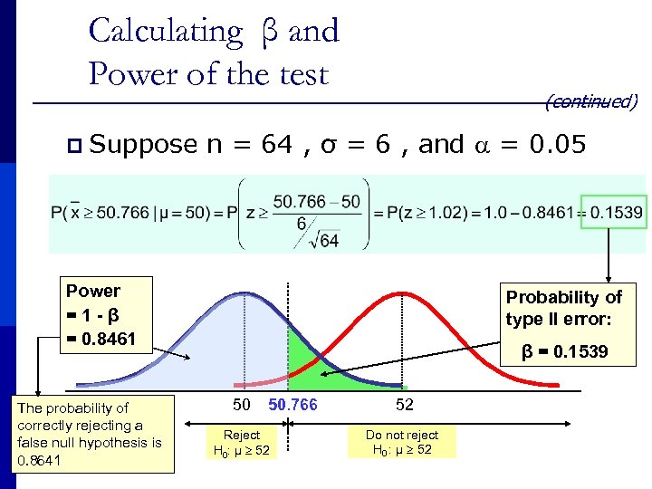
Calculating β and Power of the test (continued) p Suppose n = 64 , σ = 6 , and = 0. 05 Power =1 -β = 0. 8461 The probability of correctly rejecting a false null hypothesis is 0. 8641 Probability of type II error: β = 0. 1539 50 50. 766 Reject H 0: μ 52 52 Do not reject H 0 : μ 52
p-value p The probability value (p-value) of a statistical hypothesis test is the probability of wrongly rejecting the null hypothesis if it is in fact true. p It is equal to the significance level of the test for which we would only just reject the null hypothesis. p The p-value is compared with the actual significance level of our test and, if it is smaller, the result is significant. if the null hypothesis were to be rejected at the 5% significance level, this would be reported as "p < 0. 05". Small p-values suggest that the null hypothesis is unlikely to be true. The smaller it is, the more convincing is the rejection of the null hypothesis. p p
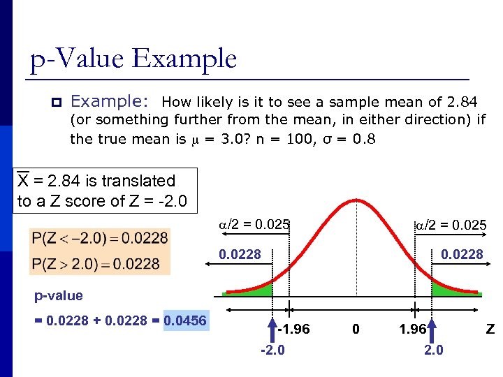
p-Value Example p Example: How likely is it to see a sample mean of 2. 84 (or something further from the mean, in either direction) if the true mean is = 3. 0? n = 100, σ = 0. 8 X = 2. 84 is translated to a Z score of Z = -2. 0 /2 = 0. 025 0. 0228 p-value = 0. 0228 + 0. 0228 = 0. 0456 -1. 96 -2. 0 0 1. 96 2. 0 Z
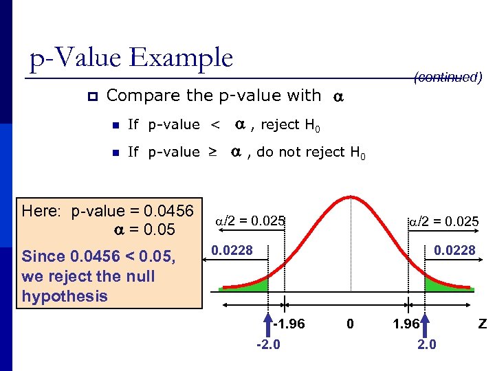
p-Value Example p (continued) Compare the p-value with n If p-value < , reject H 0 n If p-value , do not reject H 0 Here: p-value = 0. 0456 = 0. 05 Since 0. 0456 < 0. 05, we reject the null hypothesis /2 = 0. 025 0. 0228 -1. 96 -2. 0 0 1. 96 2. 0 Z
5e069707ac9288ec377e7408d9d0e79f.ppt