ba0d54e4a83055700ca9bb960aedb216.ppt
- Количество слайдов: 114

Probability and Statistics with Reliability, Queuing and Computer Science Applications: Introduction IIT Kanpur Kishor S. Trivedi Visiting Prof. Of Computer Science and Engineering, IITK Prof. Department of Electrical and Computer Engineering Duke University Durham, NC 27708 -0291 Phone: 7576 e-mail: kst@ee. duke. edu URL: www. ee. duke. edu/~kst 1
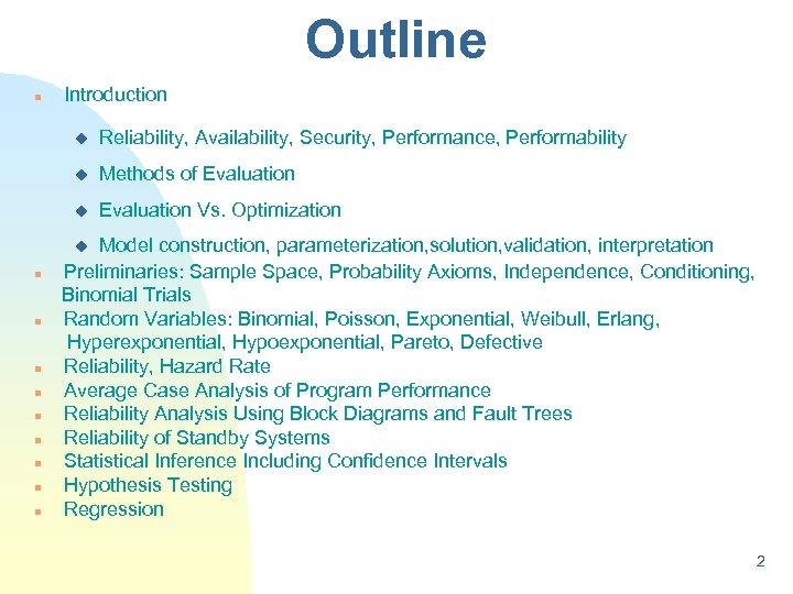
Outline n Introduction u Reliability, Availability, Security, Performance, Performability u Methods of Evaluation u Evaluation Vs. Optimization Model construction, parameterization, solution, validation, interpretation Preliminaries: Sample Space, Probability Axioms, Independence, Conditioning, Binomial Trials Random Variables: Binomial, Poisson, Exponential, Weibull, Erlang, Hyperexponential, Hypoexponential, Pareto, Defective Reliability, Hazard Rate Average Case Analysis of Program Performance Reliability Analysis Using Block Diagrams and Fault Trees Reliability of Standby Systems Statistical Inference Including Confidence Intervals Hypothesis Testing Regression u n n n n n 2
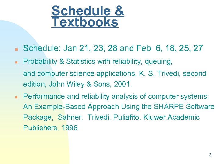
Schedule & Textbooks n Schedule: Jan 21, 23, 28 and Feb 6, 18, 25, 27 n Probability & Statistics with reliability, queuing, and computer science applications, K. S. Trivedi, second edition, John Wiley & Sons, 2001. n Performance and reliability analysis of computer systems: An Example-Based Approach Using the SHARPE Software Package, Sahner, Trivedi, Puliafito, Kluwer Academic Publishers, 1996. 3
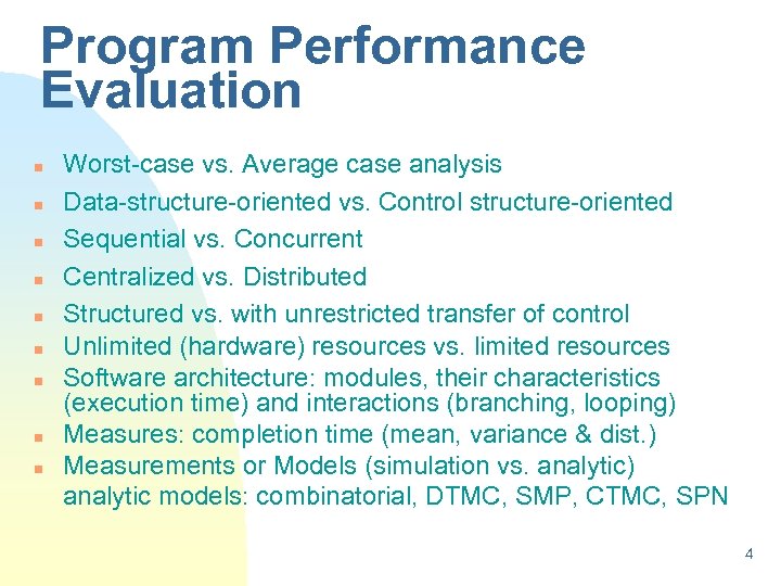
Program Performance Evaluation n n n n Worst-case vs. Average case analysis Data-structure-oriented vs. Control structure-oriented Sequential vs. Concurrent Centralized vs. Distributed Structured vs. with unrestricted transfer of control Unlimited (hardware) resources vs. limited resources Software architecture: modules, their characteristics (execution time) and interactions (branching, looping) Measures: completion time (mean, variance & dist. ) Measurements or Models (simulation vs. analytic) analytic models: combinatorial, DTMC, SMP, CTMC, SPN 4
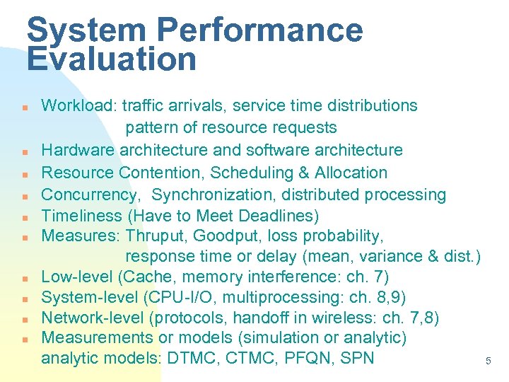
System Performance Evaluation n n Workload: traffic arrivals, service time distributions pattern of resource requests Hardware architecture and software architecture Resource Contention, Scheduling & Allocation Concurrency, Synchronization, distributed processing Timeliness (Have to Meet Deadlines) Measures: Thruput, Goodput, loss probability, response time or delay (mean, variance & dist. ) Low-level (Cache, memory interference: ch. 7) System-level (CPU-I/O, multiprocessing: ch. 8, 9) Network-level (protocols, handoff in wireless: ch. 7, 8) Measurements or models (simulation or analytic) analytic models: DTMC, CTMC, PFQN, SPN 5
System Performance Evaluation n Workload: Single vs. multiple types of requests (classes, chains) u The following items needed for each type of request: u traffic arrivals: one time vs. a stream: Poisson (Bernoulli), General renewal, IPP (IBP), MMPP(MMBP), MAP, BMAP, NHPP, Self-similar F service time distributions: Exponential (geometric), deterministic, uniform, Erlang, Hyperexponential, Hypoexponential, Phasetype, general (with finite mean and variance), Pareto F pattern of resource requests: service time distribution (or the mean) at each resource per visit, branching probabilities; often described as a DTMC (discrete-time Markov chain) and can also be seen as the behavior of an individual program F u All this information should be collected from actual measurements (if possible) followed by statistical inference 6
Software Reliability n n Black-box (measurements+ statistical inference) vs. Architecture-based approach (models) Black-box approaches treat software as a monolithic whole, considering only its interactions with external environment, without an attempt to model its internal structure With growing emphasis on reuse, software development process moves toward component-based software design White-box approach may be better to analyze a system with many software components and how they fit together 7
Software Architecture n n Software behavior with respect to the manner in which different components interact May include the information about the execution time of each component n Use control flow graph to represent architecture n Sequential program architecture modeled by F Discrete Time Markov Chain (DTMC) F Continuous Time Markov Chain (CTMC) F Semi-Markov process (SMP) 8
Failure Behavior of Components and Interfaces Failure can happen n during the execution of any component or n during the transfer of control between components Failure behavior can be specified in terms of n reliability n constant failure rate n time-dependent failure intensity 9
System Reliability/Availability n n n Faultload: fault types, fault arrivals, repair/recovery procedures and delay time distributions Hardware architecture and software architecture Minimum Resource Requirements Dynamic failures Performance/Reliability interdependence Measures: Reliability, Availability, MTTF, Downtime Low-level (Physics of failures, chip level) System-level (CPU-I/O, multiprocessing: ch. 8, 9) Software and Hardware combined together Network-level Measurements or models (simulation or analytic) analytic models: RBD, FTREE, CTMC, SPN 10
Definition of Reliability Recommendations E. 800 of the International Telecommunications Union (ITU-T) defines reliability as follows: n n “The ability of an item to perform a required function under given conditions for a given time interval. ” In this definition, an item may be a circuit board, a component on a circuit board, a module consisting of several circuit boards, a base transceiver station with several modules, a fiber-optic transport-system, or a mobile switching center (MSC) and all its subtending network elements. The definition includes systems with software. n 11
Definition of Availability is closely related to reliability, and is also defined in ITU-T Recommendation E. 800 as follows: [1] n "The ability of an item to be in a state to perform a required function at a given instant of time or at any instant of time within a given time interval, assuming that the external resources, if required, are provided. " An important difference between reliability and availability is that reliability refers to failure-free operation during an interval, while availability refers to failure-free operation at a given instant of time, usually the time when a device or system is first accessed to provide a required function or service n 12
High Reliability/Availability/Safety n Traditional applications (long-life/life-critical/safety-critical) u Space missions, aircraft control, defense, nuclear systems n New applications (non-life-critical/non-safety-critical, business critical) u Banking, airline reservation, e-commerce applications, web-hosting, telecommunication n Scientific applications (non-critical) 13
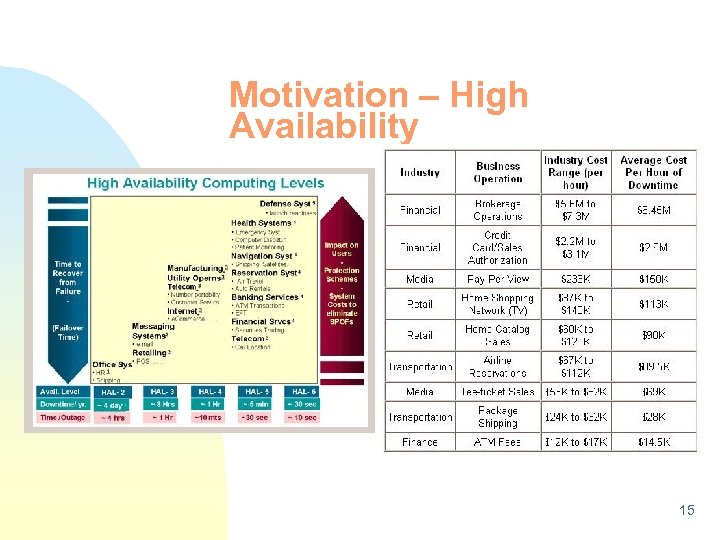
Motivation: High Availability Scott Mc. Nealy, Sun Microsystems Inc. n "We're paying people for uptime. The only thing that really matters is uptime, uptime and uptime. I want to get it down to a handful of times you might want to bring a Sun computer down in a year. I'm spending all my time with employees to get this design goal” SUN Microsystems – Sun. UP & RASCAL program for highavailability Motorola - 5 NINES Initiative HP, Cisco, Oracle, SAP - 5 nines: 5 minutes Alliance IBM – Cornhusker clustering technology for high-availability, e. Liza, autonomic computing Microsoft – Trustable computing initiative John Hennessey – in IEEE Computer Microsoft – Regular full page ad on 99. 999% availability in USA Today u n n n n 14
Motivation – High Availability 15
Need for a new term n n n Reliability is used in a generic sense Reliability used as a precisely defined mathematical function To remove confusion, IFIP WG 10. 4 has proposed Dependability as an umbrella term 16
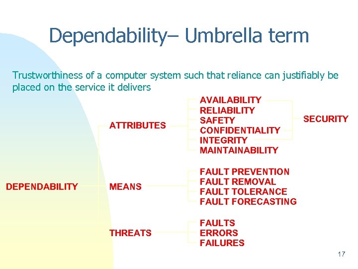
Dependability– Umbrella term Trustworthiness of a computer system such that reliance can justifiably be placed on the service it delivers ATTRIBUTES DEPENDABILITY AVAILABILITY RELIABILITY SAFETY CONFIDENTIALITY INTEGRITY MAINTAINABILITY MEANS FAULT PREVENTION FAULT REMOVAL FAULT TOLERANCE FAULT FORECASTING THREATS FAULTS ERRORS FAILURES SECURITY 17
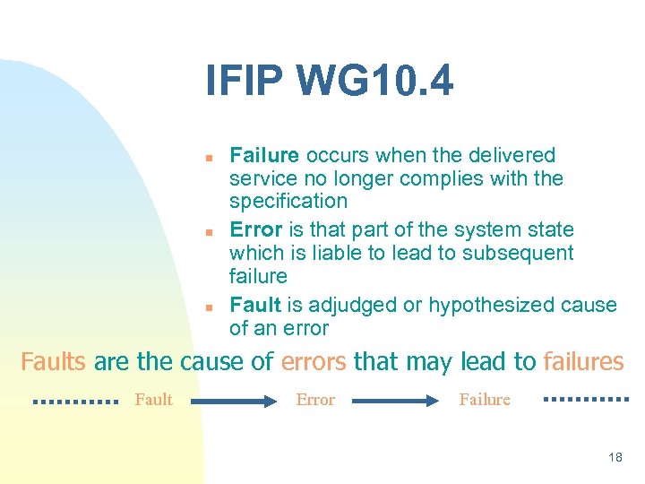
IFIP WG 10. 4 n n n Failure occurs when the delivered service no longer complies with the specification Error is that part of the system state which is liable to lead to subsequent failure Fault is adjudged or hypothesized cause of an error Faults are the cause of errors that may lead to failures Fault Error Failure 18
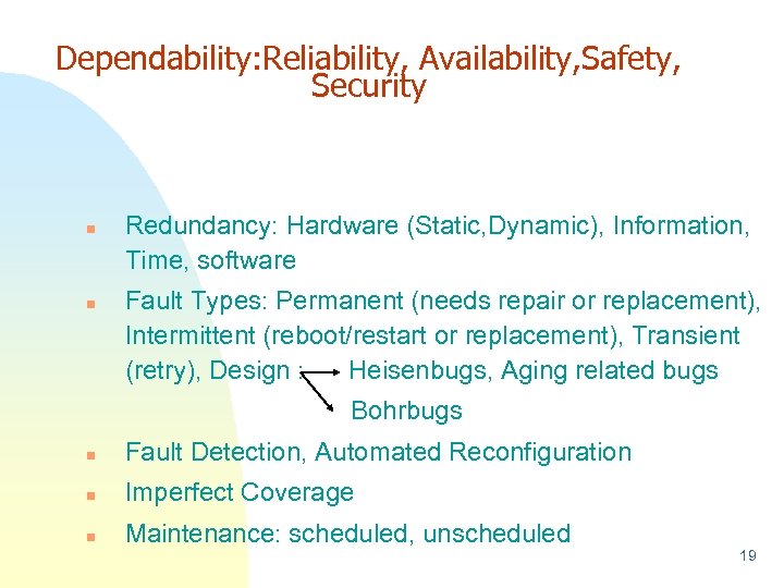
Dependability: Reliability, Availability, Safety, Security n n Redundancy: Hardware (Static, Dynamic), Information, Time, software Fault Types: Permanent (needs repair or replacement), Intermittent (reboot/restart or replacement), Transient (retry), Design : Heisenbugs, Aging related bugs Bohrbugs n Fault Detection, Automated Reconfiguration n Imperfect Coverage n Maintenance: scheduled, unscheduled 19
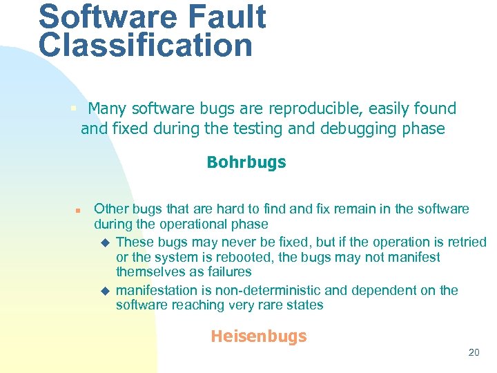
Software Fault Classification § Many software bugs are reproducible, easily found and fixed during the testing and debugging phase Bohrbugs n Other bugs that are hard to find and fix remain in the software during the operational phase u These bugs may never be fixed, but if the operation is retried or the system is rebooted, the bugs may not manifest themselves as failures u manifestation is non-deterministic and dependent on the software reaching very rare states Heisenbugs 20
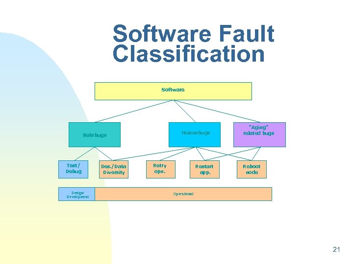
Software Fault Classification Software Heisenbugs Bohrbugs Test/ Debug Design/ Development Des. /Data Diversity Retry opn. Restart app. “Aging” related bugs Reboot node Operational 21
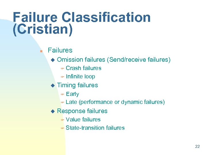
Failure Classification (Cristian) n Failures u Omission failures (Send/receive failures) Crash failures F Infinite loop F u Timing failures Early F Late (performance or dynamic failures) F u Response failures Value failures F State-transition failures F 22
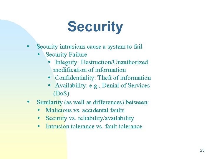
Security • Security intrusions cause a system to fail • • Security Failure • Integrity: Destruction/Unauthorized modification of information • Confidentiality: Theft of information • Availability: e. g. , Denial of Services (Do. S) Similarity (as well as differences) between: • Malicious vs. accidental faults • Security vs. reliability/availability • Intrusion tolerance vs. fault tolerance 23
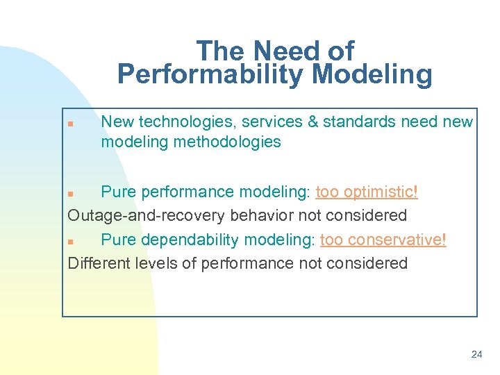
The Need of Performability Modeling n New technologies, services & standards need new modeling methodologies Pure performance modeling: too optimistic! Outage-and-recovery behavior not considered n Pure dependability modeling: too conservative! Different levels of performance not considered n 24
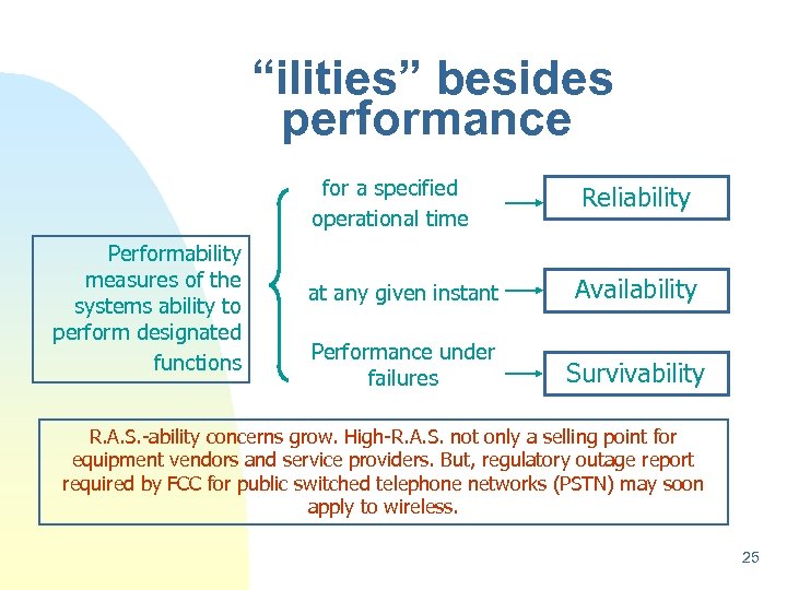
“ilities” besides performance for a specified operational time Performability measures of the systems ability to perform designated functions Reliability at any given instant Availability Performance under failures Survivability R. A. S. -ability concerns grow. High-R. A. S. not only a selling point for equipment vendors and service providers. But, regulatory outage report required by FCC for public switched telephone networks (PSTN) may soon apply to wireless. 25
Evaluation vs. Optimization n n Evaluation of system for desired measures given a set of parameters Sensitivity Analysis Bottleneck analysis u Reliability importance u n Optimization Static: Linear, integer, geometric, nonlinear, multiobjective; constrained or unconstrained u Dynamic: Dynamic programming, Markov decision process, semi-Markov decision process u 26
PURPOSE OF EVALUATION n Understanding a system u Observation Operational environment Controlled environment u Reasoning A model is a convenient abstraction n Predicting behavior of a system u Need a model u Accuracy based on degree of extrapolation 27
PURPOSE OF EVALUATION (Continued) These famous quotes bring out the difficulty of prediction based on models: n “All Models are Wrong; Some Models are Useful” George Box n “Prediction is fine as long as it is not about the future” Mark Twain 28
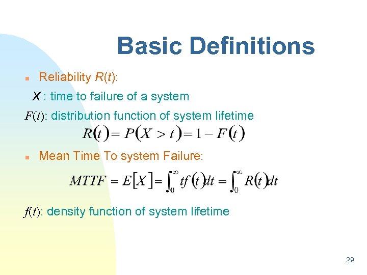
Basic Definitions n Reliability R(t): X : time to failure of a system F(t): distribution function of system lifetime n Mean Time To system Failure: f(t): density function of system lifetime 29
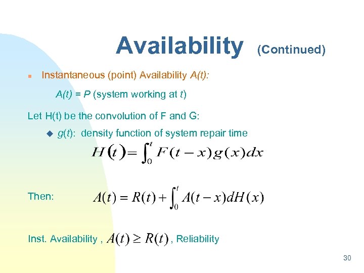
Availability n (Continued) Instantaneous (point) Availability A(t): A(t) = P (system working at t) Let H(t) be the convolution of F and G: u g(t): density function of system repair time Then: Inst. Availability , , Reliability 30
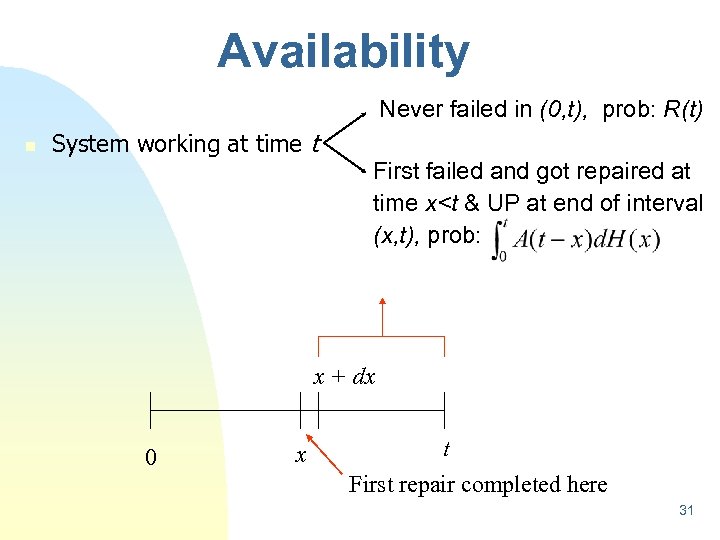
Availability Never failed in (0, t), prob: R(t) n System working at time t First failed and got repaired at time x<t & UP at end of interval (x, t), prob: x + dx 0 x t First repair completed here 31
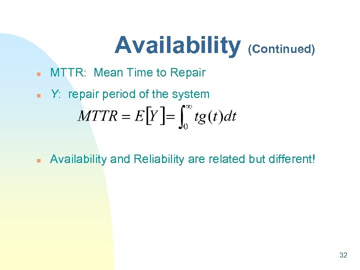
Availability (Continued) n MTTR: Mean Time to Repair n Y: repair period of the system n Availability and Reliability are related but different! 32
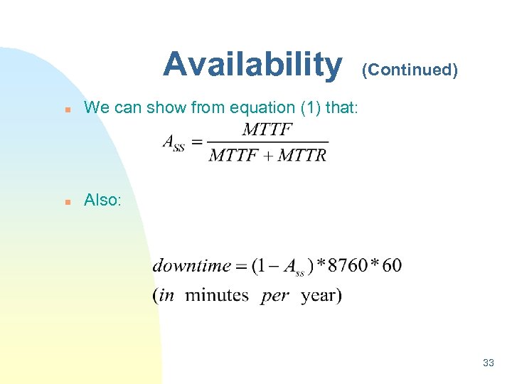
Availability n We can show from equation (1) that: n (Continued) Also: 33
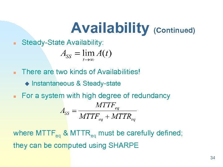
Availability (Continued) n Steady-State Availability: n There are two kinds of Availabilities! u n Instantaneous & Steady-state For a system with high degree of redundancy where MTTFeq & MTTReq must be carefully defined; they can be computed using SHARPE 34
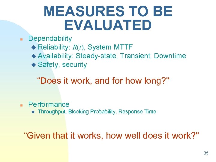
MEASURES TO BE EVALUATED n Dependability u Reliability: R(t), System MTTF u Availability: Steady-state, Transient; Downtime u Safety, security “Does it work, and for how long? '' n Performance u Throughput, Blocking Probability, Response Time “Given that it works, how well does it work? '' 35
MEASURES TO BE EVALUATED (Continued) n Composite Performance and Dependability “How much work will be done(lost) in a given interval including the effects of failure/repair/contention? '' n Need Techniques and Tools That Can Evaluate u Performance, Combinations Dependability and Their 36
Methods of EVALUATION n Measurement-Based Most believable, most expensive Not always possible or cost effective during system design u n Statistical techniques are very important here Model-Based 37
Methods of EVALUATION (Continued) n Model-Based Less believable, Less expensive 1. Discrete-Event Simulation vs. Analytic 2. State-Space Methods vs. Non-State-Space Methods 3. Hybrid: Simulation + Analytic (SPNP) 4. State Space + Non-State Space (SHARPE) 38
Methods of EVALUATION (Continued) n Measurements + Models Vaidyanathan et al ISSRE 99 39
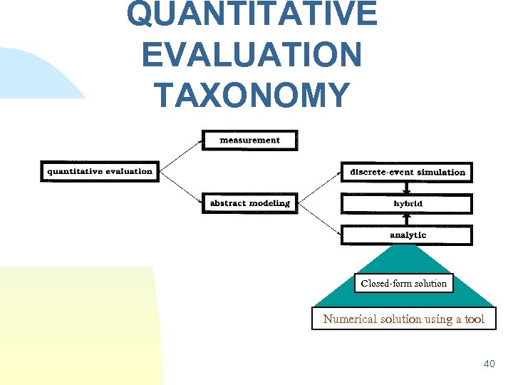
QUANTITATIVE EVALUATION TAXONOMY Closed-form solution Numerical solution using a tool 40
Note that n Both measurements & simulations imply statistical analysis of outputs (ch. 10, 11) Statistical inference u Hypothesis testing u Design of experiments u Analysis of variance u Regression (linear, nonlinear) u n n Distribution driven simulation requires generation of random deviates (variates) (ch. 3, 4, 5) Probability and Statistics are different yet highly related Probability models need inputs that generally come from measurement data (followed by statistical inference) Statistics in turn uses probability theory 41
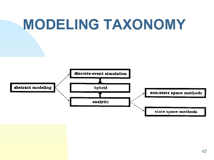
MODELING TAXONOMY 42
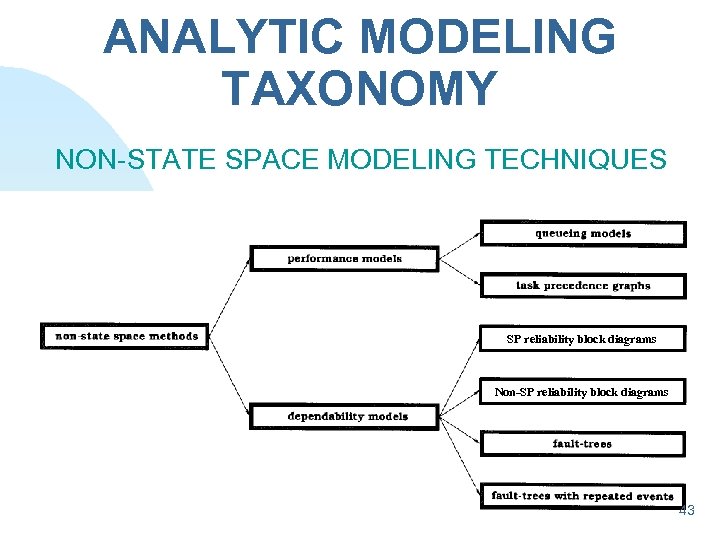
ANALYTIC MODELING TAXONOMY NON-STATE SPACE MODELING TECHNIQUES SP reliability block diagrams Non-SP reliability block diagrams 43
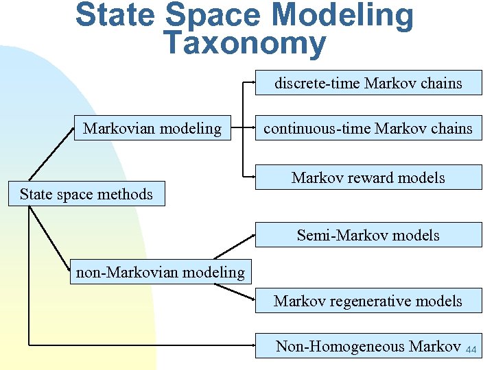
State Space Modeling Taxonomy discrete-time Markov chains Markovian modeling State space methods continuous-time Markov chains Markov reward models Semi-Markov models non-Markovian modeling Markov regenerative models Non-Homogeneous Markov 44
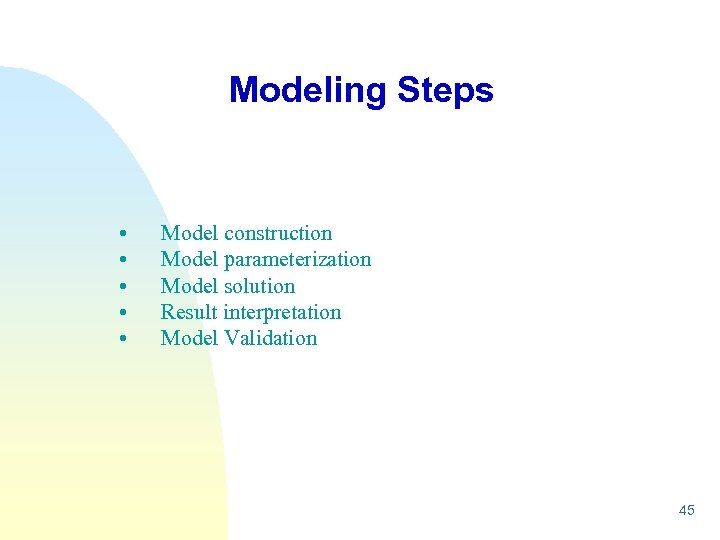
Modeling Steps • • • Model construction Model parameterization Model solution Result interpretation Model Validation 45
n MODELING AND MEASUREMENTS: INTERFACES Models Measurements supply Input Parameters to (Model Calibration or Parameterization) Confidence Intervals should be obtained Boeing, Draper, Union Switch projects n Model Sensitivity Analysis can suggest which Parameters to Measure More Accurately: Blake, Reibman and Trivedi: SIGMETRICS 1988. 46
n MODELING AND MEASUREMENTS: INTERFACES Model Validation 1. Face Validation 2. Input-Output Validation 3. Validation of Model Assumptions (Hypothesis Testing) n Rejection of a hypothesis regarding model assumption based on measurement data leads to an improved model 47
MODELING AND MEASUREMENTS: INTERFACES n Model Structure Based on Measurement Data u Hsueh, Iyer and Trivedi; IEEE TC, April 1988 u Gokhale et al, IPDS 98; u Vaidyanathan et al, ISSRE 99 48

MODELING TAXONOMY 49

ANALYTIC MODELING TAXONOMY NON-STATE SPACE MODELING TECHNIQUES SP reliability block diagrams Non-SP reliability block diagrams 50
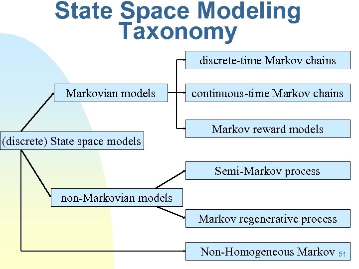
State Space Modeling Taxonomy discrete-time Markov chains Markovian models (discrete) State space models continuous-time Markov chains Markov reward models Semi-Markov process non-Markovian models Markov regenerative process Non-Homogeneous Markov 51
MODELING THROUGHOUT SYSTEM LIFECYCLE n System Specification/Design Phase Answer “What-if Questions'' u Compare design alternatives (Bedrock, Wireless handoff) u Performance-Dependability Trade-offs (Wireless Handoff) u Design Optimization (optimizing the number of guard channels) 52
MODELING THROUGHOUT SYSTEM LIFECYCLE (Continued) n Design Verification Phase Use Measurements + Models E. g. Fault/Injection + Availability Model Union Switch and Signals, Boeing, Draper n Configuration Selection Phase: DEC, HP n System Operational Phase: IDEN Project Workload based adaptive rejuvenation • It is fun! 53
MODELER'S DILEMMA Should I Use Discrete-Event Simulation? n Point Estimates and Confidence Intervals n How many simulation runs are sufficient? n What Specification Language to use? u C, SIMULA, SIMSCRIPT, MODSIM, GPSS, RESQ, SPNP v 6, Bones, SES workbench, ns, opnet 54
MODELER'S DILEMMA (Continued) n Simulation: + Detailed System Behavior including non-exponential behavior + Performance, Dependability and Performability Modeling Possible - Long Execution Time (Variance Reduction Possible) u Importance Sampling, importance splitting, regenerative simulation. u Parallel and Distributed Simulation - Many users in practice do not realize the need to calculate confidence intervals 55
MODELER'S DILEMMA (Continued) Should I Use Non-State-Space Methods? n Also Known as Combinatorial Models n Model Solved Without Generating State Space n Use: Order Statistics, Mixing, Convolution (chapters 1 -5) n Common Dependability Model Types: also called Combinatorial Models u Series-Parallel Reliability Block Diagrams u Non-Series-Parallel Block Diagrams (or Reliability Graphs) u Fault-Trees Without Repeated Events u Fault-Trees With Repeated Events 56
Combinatorial analytic models n Reliability block diagrams, Fault trees and Reliability graphs u Commonly used for reliability and availability u These model types are similar in that they capture conditions that make a system fail in terms of the structural relationships between the system components. 57
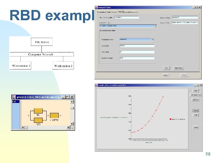
RBD example 58
Combinatorial Models n n Combinatorial modeling techniques like RBDs and FTs are easy to use and assuming statistical independence solve for system availability and system MTTF Each component can have attached to it u. A probability of failure u A failure rate u A distribution of time to failure u Steady-state and instantaneous unavailability 59
Non-State Space Modeling Techniques n Possible to compute (given component failure/repair rates: ) u. System Reliability u. System Availability (Steady-state, instantaneous) u. Downtime u. System MTTF 60
Non-State Space Modeling Techniques (Continued) n Assuming: u u n Failures are statistically independent As many repair units as needed Relatively good algorithms are available for solving such models so that 100 component systems can be handled. 61
Non-State Space Modeling Techniques (Continued) n Common Model Types: Performance u Series-Parallel Task Precedence Graphs u Product-Form Queuing Networks + Easy specification, fast computation, no distributional assumption + Can easily solve models with 100’s of components 62
Combinatorial Modeling (Continued) n - These models can be solved using fast algorithms assuming stochastic independence between system components. Systems with several hundred components can be handled. u Sum of disjoint products (SDP) algorithms u Binary decision diagrams (BDD) algorithms u Factoring (conditioning) algorithms u Series-parallel composition algorithm Failure/Repair Dependencies are often present; RBDs, FTREEs cannot easily handle these u (e. g. , shared repair, warm/cold spares, imperfect coverage, non- zero switching time, travel time of repair person, reliability with repair) 63
Markov chain n To model more complicated interactions between components, use other kinds of models like Markov chains or more generally state space models. n Many examples of dependencies among system components have been observed in practice and captured by Markov models. 64
State-Space-Based Models n n States and labeled state transitions State can keep track of: u Number of functioning resources of each type u States of recovery for each failed resource u Number of tasks of each type waiting at each resource u Allocation of resources to tasks n A transition: u Can occur from any state to any other state u Can represent a simple or a compound event 65
State-Space-Based Models (Continued) n Transitions between states represent the change of the system state due to the occurrence of an event n Drawn as a directed graph n Transition label: u Probability: homogeneous discrete-time Markov chain (DTMC) u Rate: homogeneous continuous-time Markov chain (CTMC) u Time-dependent rate: non-homogeneous CTMC u Distribution function: semi-Markov process (SMP) u Two distribution functions; Markov regenerative process (MRGP) 66
MODELER'S DILEMMA (Continued) Should I Use Markov Models? State-Space-Based Methods + Model Fault-Tolerance and Recovery/Repair + Model Dependencies + Model Contention for Resources + Model Concurrency and Timeliness + Generalize to Markov Reward Models for Modeling Degradable Performance 67
MODELER'S DILEMMA (Continued) Should I Use Markov Models? + Generalize to Markov Regenerative Models for Allowing Generally Distributed Event Times + Generalize to Non-Homogeneous Markov Chains for Allowing Weibull Failure Distributions + Performance, Availability and Performability Modeling Possible - Large (Exponential) State Space 68
IN ORDER TO FULFILL OUR GOALS n n Modeling Performance, Availability and Performability Modeling Complex Systems We Need n Automatic Generation and Solution of Large Markov Reward Models 69
IN ORDER TO FULFILL OUR GOALS (Continued) n Facility for State Truncation, Hierarchical composition of Non-State-Space and State-Space Models, Fixed-Point Iteration u n n There are Two Tools that Potentially meet these Goals Stochastic Petri Net Package (SPNP) Symbolic Hierarchical Automated Reliability and Performance Evaluator (SHARPE) 70
Model-based Performance/Dependability evaluation n Choice of the model type is dictated by: u Measures of interest u Level of detailed system behavior to be represented u Ease of model specification and solution u Representation u Access power of the model type to suitable tools or toolkits 71
Difficulty in Modeling using Markov chains The Markov chains tend to be large and complex leading too: u Model generation problem Use automated means of generating the Markov chains: Stochastic Petri Nets, Stochastic Reward Nets 72
Difficulty in Modeling using Markov chains (Continued) n Model solution problem Use sparse storage for the matrices Use sparsity preserving solution methods u Sucessive Overrelaxation, u Gauss-Seidel, u Uniformization, u ODE-solution methods 73
Markov Reward Models (MRMs) n Modeling any system with a pure reliability / availability model can lead to incomplete, or, at least, less precise results. u Gracefully degrading systems may be able to survive the failure of one or more of their active components and continue to provide service at a reduced level. u Markov reward model is commonly used technique for the modeling of gracefully degradable system 74
State-Space-Based Models n Use also the following model types: u Markov chains & Markov reward models u semi-Markov & Markov regenerative processes u Stochastic reward nets or generalized stochastic Petri nets. F SRN & GSPN models are transformed into Markov chains for analysis. F Only model types (in SHARPE) that requires a conversion to a different model (Markov chain) to be solved. 75
Summary- Modeling Techniques n n Combinatorial techniques like RBDs and FTREEs are easy to use and solve Combinatorial models cannot easily represent intricate dependencies State space based models like Markov chains can handle dependencies State space explosion problem u Use automated generation methods: stochastic Petri nets u Concurrency, contention and conditional branching easily modeled with Petri nets. 76
Hierarchy used n State space explosion can be handled in two ways: Large model tolerance must apply to specification, storage and solution of the model. If the storage and solution problems can be solved, the specification problem can be solved by using more concise (and smaller) model specifications that can be automatically transformed into Markov models. u Large models can be avoided by using hierarchical (Multilevel) model composition. u 77
LARGENESS AVOIDANCE n Non-State-Space methods u Reliability block diagrams u Fault-trees u Product-Form n Queuing Networks Approximate solutions u State Truncation SAVE, SPNP, ASSIST (Kantz and Trivedi: PNPM 91) 78
VAXcluster example Hierarchie: Diode on top, CTMC at bottom Storage model 79
Approximate Availability Model for the Processing Subsystem 80
Availability Model for the VAXcluster Storage Subsystem Reliability block diagram for the storage system 81
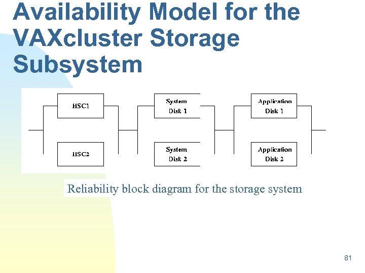
A novel availability model for VAXclusters with large storage subsystems. n n The configuration shown consists of two HSCs, and a set of disks. The disks are further classified into two system disks and two application disks. The operating system resides on the system disk, and the user accounts and other application software on the application disks. Further, it is assumed that the disks are shadowed and dual pathed and ported between the two HSCs. A disk dual pathed between two HSCs can be accessed cluster-wide in a coordinated way 82 through either HSC. In case, one of the HSC fails,
Assumptions n The model assumed that each component in the block diagram has its own repair facility. n The repair time is a 2 -stage hypoexponentially distributed random variable with the first phase being the travel time and the second phase being the actual repair time. 83
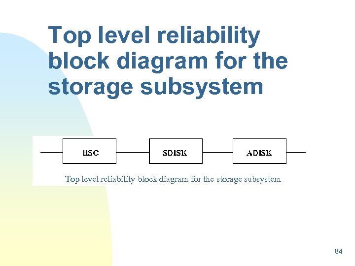
Top level reliability block diagram for the storage subsystem 84
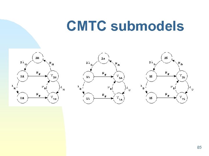
CMTC submodels 85
Assumptions n In the second improved model, we removed the assumption of independent repair. Instead, it is assumed that a repair facility is shared within a subsystem. n The storage system is now assumed as a two-level hierarchical model. The bottom level consists of three independent CTMC models, namely HSC, SDisk and ADisk, representing the HSC, system disk and application disk subsystems respectively. n The top level consists of a reliability block diagram 86
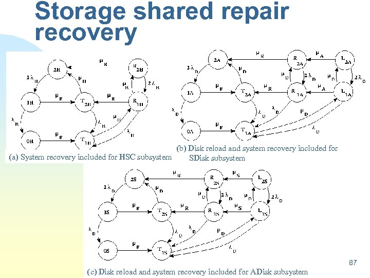
Storage shared repair recovery (b) Disk reload and system recovery included for (a) System recovery included for HSC subsystem SDisk subsystem 87 (c) Disk reload and system recovery included for ADisk subsystem
Assumptions n In the third approximation we took into account disk reload and system recovery. This takes into account the following activities. n When a disk subsystem experiences a failure, data on the disk may be corrupted or lost. After the disk is repaired the data is reloaded on to the disk from an external source, such as a backup disk or tape. While the reload is a local activity of a disk subsystem, recovery is a global system-wide 88
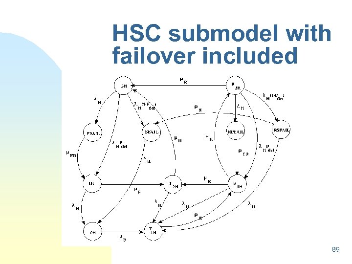
HSC submodel with failover included 89
An Introduction to SHARPE software tool 90
n n n Overview of SHARPE: Symbolic-Hierarchical Automated Reliability and Performance Evaluator Well-known modeling tool (Installed at over 300 Sites; companies and universities) Combines flexibility of Markov models and efficiency of combinatorial models Ported to most architectures and operating systems Used for Education, Research, Engineering Practice 91
Overview of SHARPE (cont. ) n Graphical User Interface is available n Used for analysis of performance(traffic), dependability and performability n Hierarchy facilitates largeness & stiffness avoidance n Steady-state as well as transient analysis n Written in C language n Used as an engine by several other tools 92
SHARPE - new features n Many more built in distributions n Ability to easily specify structured Markov chains (Loop feature) n Ability to print models and outputs 93
New Features n n n n Equivalent mean time to system failure and equivalent mean time to system repair implemented for Markov chains and RBDs BDD algorithms implemented for FTs and RGs Steady-state computation of MRGP models Stochastic reward net is available as a model type Fast MTTF algorithm implemented for Markov chain Mathematica used for some fully symbolic computations GUI implemented 94
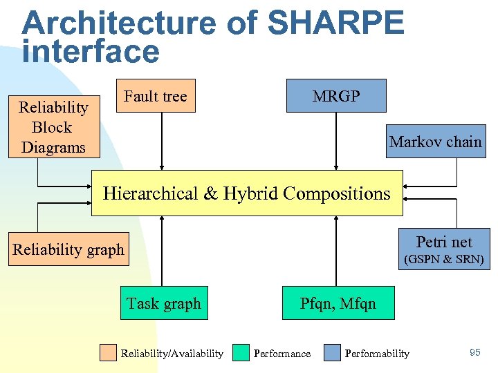
Architecture of SHARPE interface Reliability Block Diagrams Fault tree MRGP Markov chain Hierarchical & Hybrid Compositions Petri net Reliability graph (GSPN & SRN) Task graph Reliability/Availability Pfqn, Mfqn Performance Performability 95
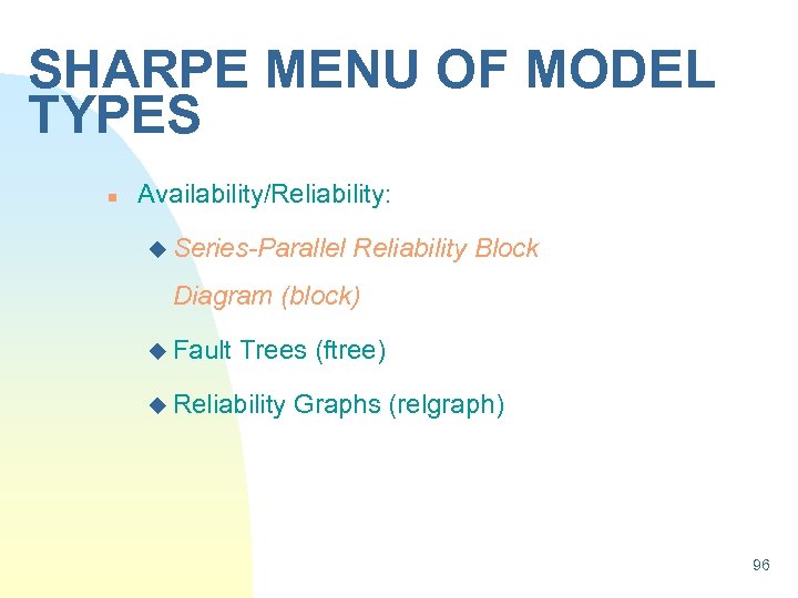
SHARPE MENU OF MODEL TYPES n Availability/Reliability: u Series-Parallel Reliability Block Diagram (block) u Fault Trees (ftree) u Reliability Graphs (relgraph) 96
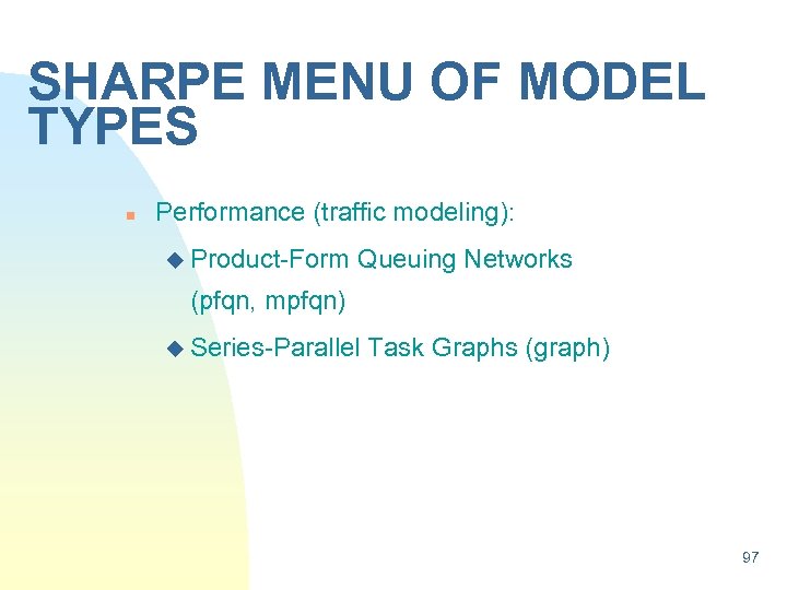
SHARPE MENU OF MODEL TYPES n Performance (traffic modeling): u Product-Form Queuing Networks (pfqn, mpfqn) u Series-Parallel Task Graphs (graph) 97
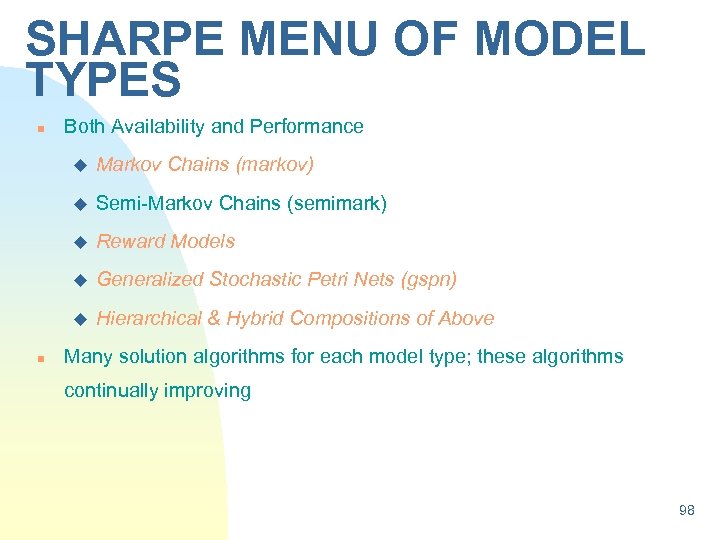
SHARPE MENU OF MODEL TYPES n Both Availability and Performance u u Semi-Markov Chains (semimark) u Reward Models u Generalized Stochastic Petri Nets (gspn) u n Markov Chains (markov) Hierarchical & Hybrid Compositions of Above Many solution algorithms for each model type; these algorithms continually improving 98
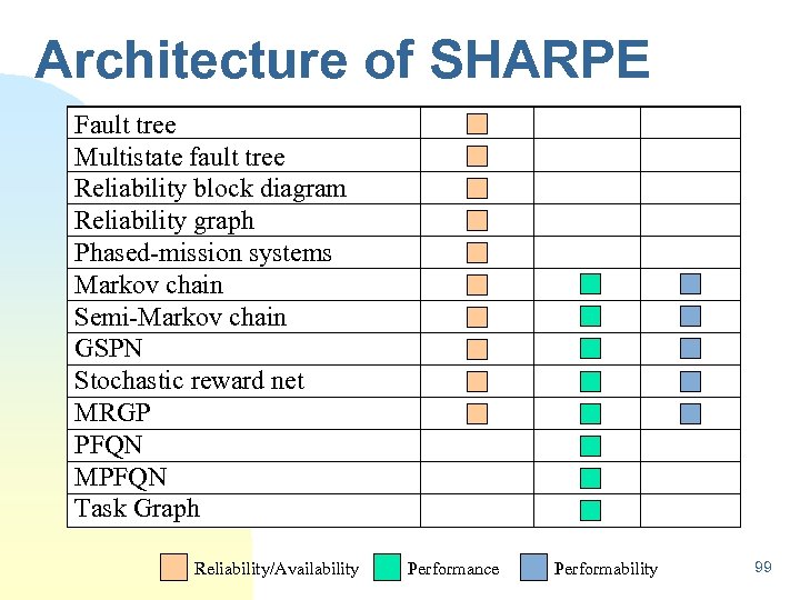
Architecture of SHARPE Fault tree Multistate fault tree Reliability block diagram Reliability graph Phased-mission systems Markov chain Semi-Markov chain GSPN Stochastic reward net MRGP PFQN MPFQN Task Graph Reliability/Availability Performance Performability 99
State Space Explosion n State space explosion can be handled in two ways: Large model tolerance must apply to specification, storage and solution of the model. If the storage and solution problems can be solved, the specification problem can be solved by using more concise (and smaller) model specifications that can be automatically transformed into Markov models (GSPN and SRN models). u Large models can be avoided by using hierarchical model composition. u n Ability of SHARPE to combine results from different kinds of models u Possibility to use state-space methods for those parts of a system that require them, and use non-state-space methods for the more “well-behaved” parts of the system. 100
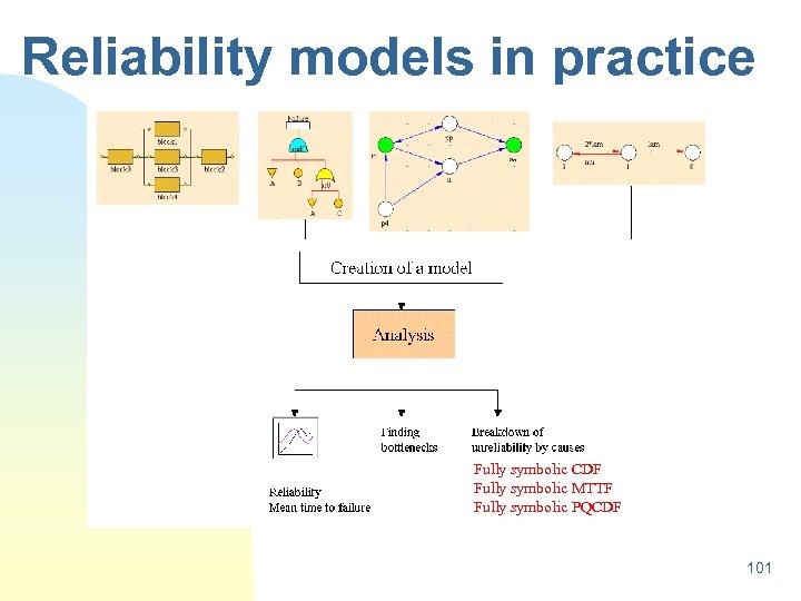
Reliability models in practice Fully symbolic CDF Fully symbolic MTTF Fully symbolic PQCDF 101
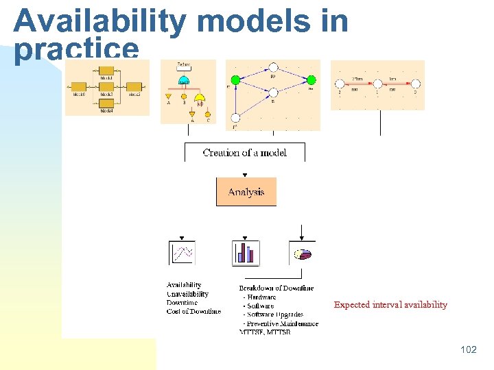
Availability models in practice Expected interval availability 102

RBD example 103
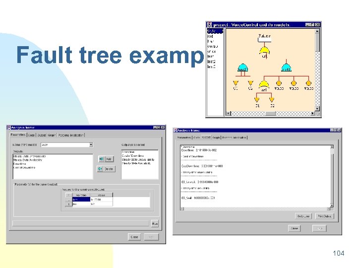
Fault tree example 104
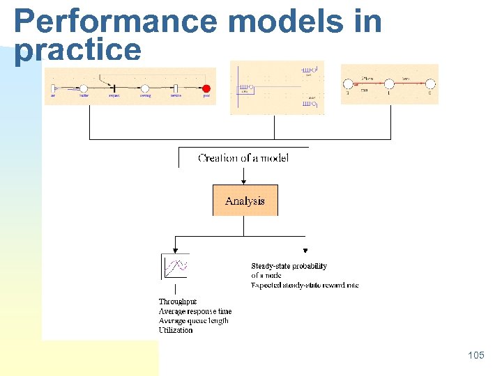
Performance models in practice 105
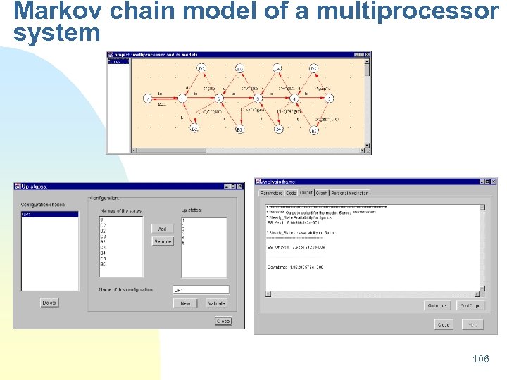
Markov chain model of a multiprocessor system 106
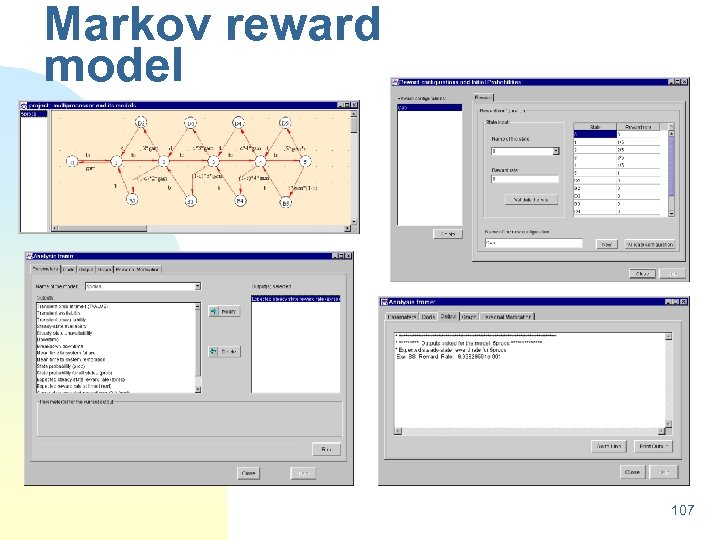
Markov reward model 107
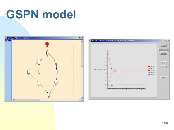
GSPN model 108
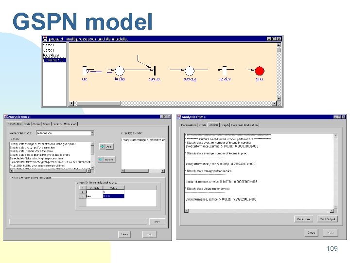
GSPN model 109
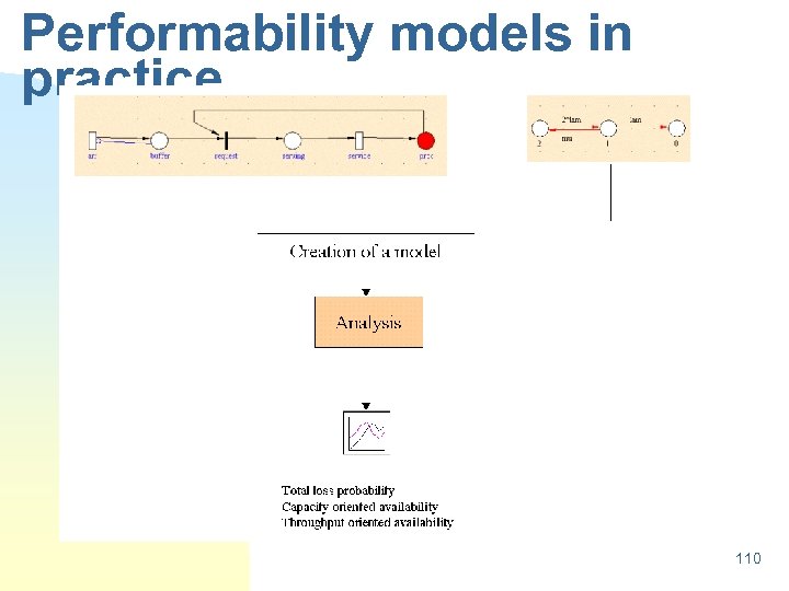
Performability models in practice 110
Possible outputs n n n Availability, Unavailability and Downtime Cost of downtime Mean Time to System Failure, Mean Time to System Repair Downtime breakdown into Hardware, Software & Upgrade Breakdown of downtime by states for Markov chain models, by blocks for Reliability block diagram models. Sensitivity Analysis, Strategy to improve the availability of the systems. 111
SHARPE - references n Performance and Reliability Analysis of Computer Systems, Robin Sahner, Kishor Trivedi, A. Puliafito, Kluwer Academic Press, 1996, Red book n Reliability and Performability Modeling using SHARPE 2000, C. Hirel, R. Sahner, X. Zang, K. Trivedi Computer performance evaluation: Modelling tools and techniques; 11 th International Conference; TOOLS 2000, Schaumburg, Il. , USA, March 2000. 112
ADVANTAGES OF THE APPROACH n Pick a Natural Model Type for a Given Application (No Retrofitting Required) n Use a Natural Model Type for a Portion of a Model (Encourages Hybrid and Hierarchical Composition) 113
ADVANTAGES OF THE APPROACH n Except for gspn and srn Models, No Internal Conversion Done Appropriate Solution Algorithm for Each Model Type i. e. , Hierarchy for Solution as well as Specification n Pedagogic Advantages n Multi-Version Modeling n Step-Wise Refinement in Modeling 114
ba0d54e4a83055700ca9bb960aedb216.ppt