3f5c3f93a19e684d37579f71ad9395a8.ppt
- Количество слайдов: 131
Probability and Discrete Random Variable
Probability
What is Probability? • When we talk about probability, we are talking about a (mathematical) measure of how likely it is for some particular thing to happen • Probability deals with chance behavior – We study outcomes, or results of experiments – Each time we conduct an experiment, we may get a different result
Why study Probability? • Descriptive statistics - describing and summarizing sample data, deals with data as it is • Probability - Modeling the probabilities for sample results to occur in situations in which the population is known • The combination of the two will let us do our inferential statistics techniques.
Objectives 1. Learn the basic concepts of probability 2. Understand the rules of probabilities 3. Compute and interpret probabilities using the empirical method 4. Compute and interpret probabilities using the classical method 5. Compute the probabilities for the compound events.
Sample Space & Outcomes • Some definitions – An experiment is a repeatable process where the results are uncertain – An outcome is one specific possible result – The set of all possible outcomes is the sample space denoted by a capital letter S • Example – Experiment … roll a fair 6 sided die – One of the outcomes … roll a “ 4” – The sample space … roll a “ 1” or “ 2” or “ 3” or “ 4” or “ 5” or “ 6”. So, S = {1, 2, 3, 4, 5, 6} (Include all outcomes in braces {…}. )
Event • More definitions – An event is a collection of possible outcomes … we will use capital letters such as E for events – Outcomes are also sometimes called simple events … we will use lower case letters such as e for outcomes / simple events • Example (continued) – One of the events … E = {roll an even number} – E consists of the outcomes e 2 = “roll a 2”, e 4 = “roll a 4”, and e 6 = “roll a 6” … we’ll write that as {2, 4, 6}
Example Consider an experiment of rolling a die again. – There are 6 possible outcomes, e 1 = “rolling a 1” which we’ll write as just {1}, e 2 = “rolling a 2” or {2}, … – The sample space is the collection of those 6 outcomes. We write S = {1, 2, 3, 4, 5, 6} – One event of interest is E = “rolling an even number”. The event is indicated by E = {2, 4, 6}
Probability of an Event • If E is an event, then we write P(E) as the probability of the event E happening • These probabilities must obey certain mathematical rules
Probability Rule # 1 • Rule # 1 – the probability of any event must be greater than or equal to 0 and less than or equal to 1, i. e. , – It does not make sense to say that there is a -30% chance of rain – It does not make sense to say that there is a 140% chance of rain Note – probabilities can be written as decimals (0, 0. 3, 1. 0), or as percents (0%, 30%, 100%), or as fractions (3/10)
Probability Rule # 2 • Rule #2 – the sum of the probabilities of all the outcomes must equal 1. – If we examine all possible outcomes, one of them must happen – It does not make sense to say that there are two possibilities, one occurring with probability 20% and the other with probability 50% (where did the other 30% go? )
Example On the way to work Bob’s personal judgment is that he is four times more likely to get caught in a traffic jam (TJ) than have an easy commute (EC). What values should be assigned to P(TJ) and P(EC)? Solution: Given Since Which means
Probability Rule (continued) • Probability models must satisfy both of these rules • There are some special types of events – If an event is impossible, then its probability must be equal to 0 (i. e. it can never happen) – If an event is a certainty, then its probability must be equal to 1 (i. e. it always happens)
Unusual Events • A more sophisticated concept – An unusual event is one that has a low probability of occurring – This is not precise … how low is “low? • Typically, probabilities of 5% or less are considered low … events with probabilities of 5% or lower are considered unusual • However, this cutoff point can vary by the context of the problem
How To Compute the Probability? The probability of an event may be obtained in three different ways: – Theoretically (a classical approach) – Empirically (an experimental approach) – Subjectively
Compute Probability theoretically
Equally Likely Outcomes • The classical method of calculating the probability applies to situations (or by assuming the situations) where all possible outcomes have the same probability which is called equally likely outcomes • Examples – Flipping a fair coin … two outcomes (heads and tails) … both equally likely – Rolling a fair die … six outcomes (1, 2, 3, 4, 5, and 6) … all equally likely – Choosing one student out of 250 in a simple random sample … 250 outcomes … all equally likely
Equally Likely Outcomes • Because all the outcomes are equally likely, then each outcome occurs with probability 1/n where n is the number of outcomes • Examples – Flipping a fair coin … two outcomes (heads and tails) … each occurs with probability 1/2 – Rolling a fair die … six outcomes (1, 2, 3, 4, 5, and 6) … each occurs with probability 1/6 – Choosing one student out of 250 in a simple random sample … 250 outcomes … each occurs with probability 1/250
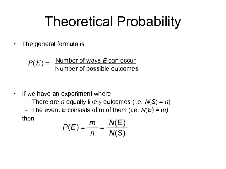
Theoretical Probability • The general formula is Number of ways E can occur Number of possible outcomes • If we have an experiment where – There are n equally likely outcomes (i. e. N(S) = n) – The event E consists of m of them (i. e. N(E) = m) then
A More Complex Example Here we consider an example of select two subjects at random instead of just one subject: Three students (Katherine (K), Michael (M), and Dana (D)) want to go to a concert but there are only two tickets available. Two of the three students are selected at random. Question 1: What is the sample space of who goes? Solution: S = {(K, M), (K, D), (M, D)} Question 2: What is the probability that Katherine goes? Solution: Because 2 students are selected at random, each outcome in the sample space has equal chance to occur. Therefore, P( Katherine goes) = 2/3.
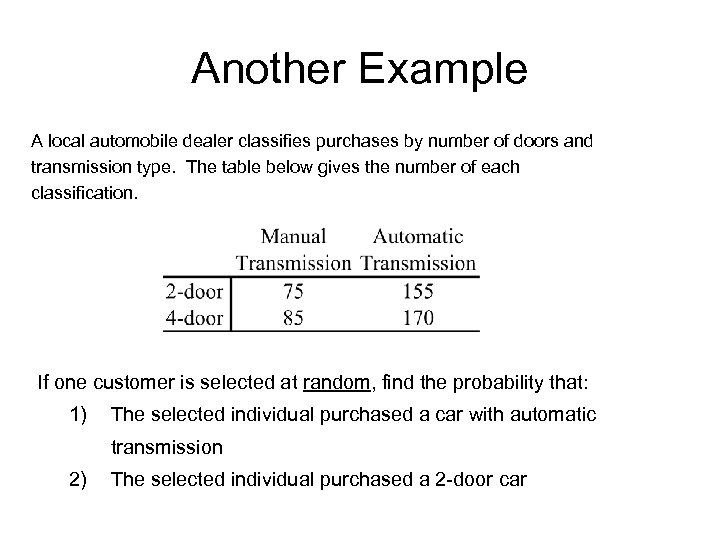
Another Example A local automobile dealer classifies purchases by number of doors and transmission type. The table below gives the number of each classification. If one customer is selected at random, find the probability that: 1) The selected individual purchased a car with automatic transmission 2) The selected individual purchased a 2 -door car
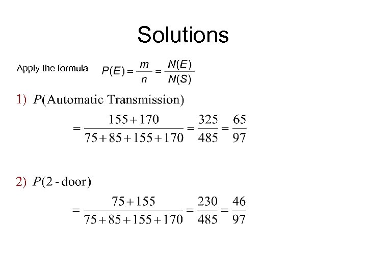
Solutions Apply the formula 1) 2)
Compute Probability empirically
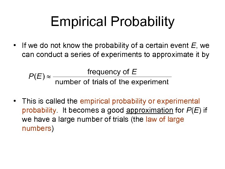
Empirical Probability • If we do not know the probability of a certain event E, we can conduct a series of experiments to approximate it by • This is called the empirical probability or experimental probability. It becomes a good approximation for P(E) if we have a large number of trials (the law of large numbers)
Example We wish to determine what proportion of students at a certain school have type A blood – We perform an experiment (a simple random sample!) with 100 students – If 29 of those students have type A blood, then we would estimate that the proportion of students at this school with type A blood is 29%
Example (continued) We wish to determine what proportion of students at a certain school have type AB blood – We perform an experiment (a simple random sample!) with 100 students – If 3 of those students have type AB blood, then we would estimate that the proportion of students at this school with type AB blood is 3% – This would be an unusual event
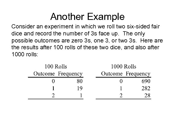
Another Example Consider an experiment in which we roll two six-sided fair dice and record the number of 3 s face up. The only possible outcomes are zero 3 s, one 3, or two 3 s. Here are the results after 100 rolls of these two dice, and also after 1000 rolls:
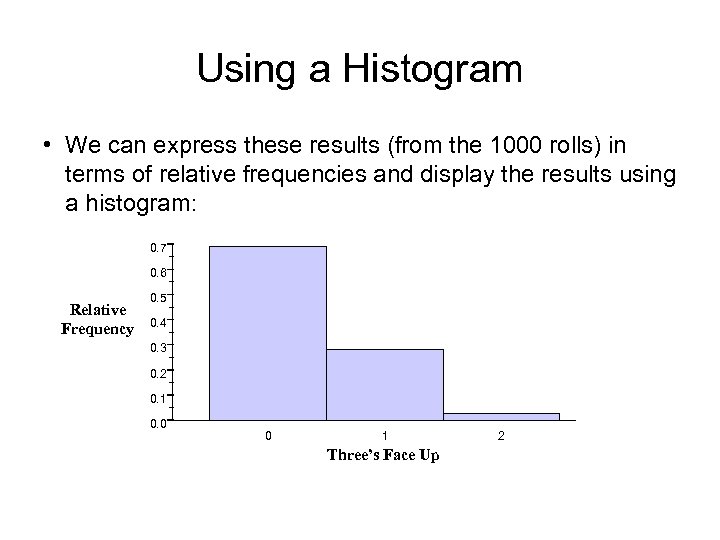
Using a Histogram • We can express these results (from the 1000 rolls) in terms of relative frequencies and display the results using a histogram: 0. 7 0. 6 Relative Frequency 0. 5 0. 4 0. 3 0. 2 0. 1 0. 0 0 1 Three’s Face Up 2
Continuing the Experiment If we continue this experiment for several thousand more rolls, the relative frequency for each possible outcome will settle down and approach to a constant. This is so called the law of large numbers.
Coin-Tossing Experiment Consider tossing a fair coin. Define the event H as the occurrence of a head. What is the probability of the event H, P(H)? • Theoretical approach – If we assume that the coin is fair, then there are two equally likely outcomes in a single toss of the coin. Intuitively, P(H) = 50%. • Empirical approach – If we do not know if the coin is fair or not. We then estimate the probability by tossing the coin many times and calculating the proportion of heads occurring. To show you the effect of applying large number of tosses on the accuracy of the estimation. What we actually do here is to toss the coin 10 times each time and repeated it 20 times. The results are shown in the next slide. We cumulate the total number of tosses over trials to compute the proportion of heads. We plot the proportions over trials in a graph as shown in the following slide. We observe that the proportion of heads tends to stabilize or settle down near 0. 5 (50%). So, the proportion of heads over larger number of tosses is a better estimate of the true probability P(H).
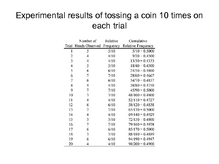
Experimental results of tossing a coin 10 times on each trial
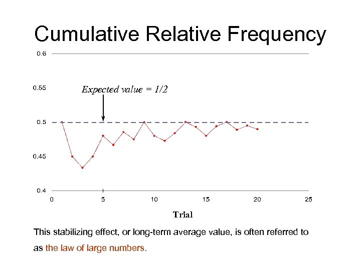
Cumulative Relative Frequency Expected value = 1/2 Trial This stabilizing effect, or long-term average value, is often referred to as the law of large numbers.
Law of Large Numbers If the number of times an experiment is repeated is increased, the ratio of the number of successful occurrences to the number of trials will tend to approach theoretical probability of the outcome for an individual trial – Interpretation: The law of large numbers says: the larger the number of experimental trials, the closer the empirical probability is expected to be to the true probability P(A)
Subjective Probability 1. Suppose the sample space elements are not equally likely and empirical probabilities cannot be used 2. Only method available for assigning probabilities may be personal judgment 3. These probability assignments are called subjective probabilities
Summary • Probabilities describe the chances of events occurring … events consisting of outcomes in a sample space • Probabilities must obey certain rules such as always being greater than or equal to 0 and less then or equal to 1. • There are various ways to compute probabilities, including empirical method and classical method for experiments with equally likely outcomes.
Compute Probabilities for Compound Events
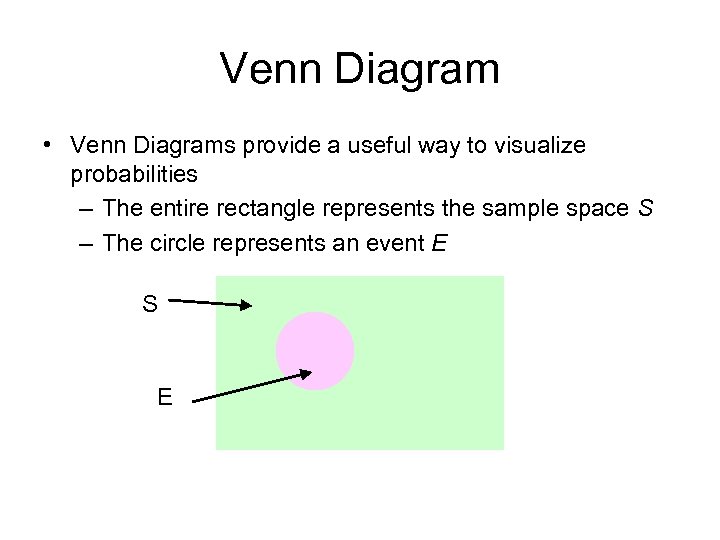
Venn Diagram • Venn Diagrams provide a useful way to visualize probabilities – The entire rectangle represents the sample space S – The circle represents an event E S E
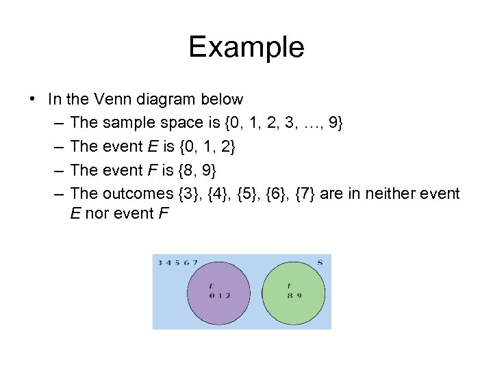
Example • In the Venn diagram below – The sample space is {0, 1, 2, 3, …, 9} – The event E is {0, 1, 2} – The event F is {8, 9} – The outcomes {3}, {4}, {5}, {6}, {7} are in neither event E nor event F
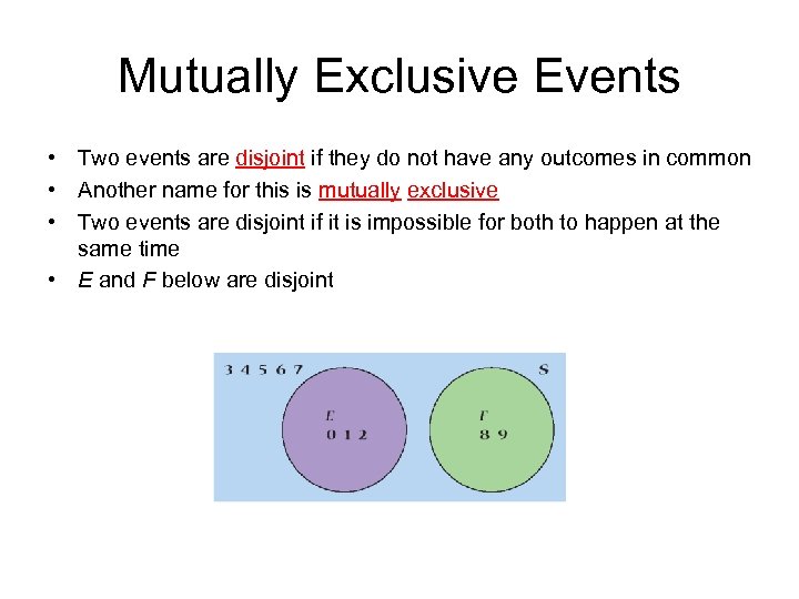
Mutually Exclusive Events • Two events are disjoint if they do not have any outcomes in common • Another name for this is mutually exclusive • Two events are disjoint if it is impossible for both to happen at the same time • E and F below are disjoint
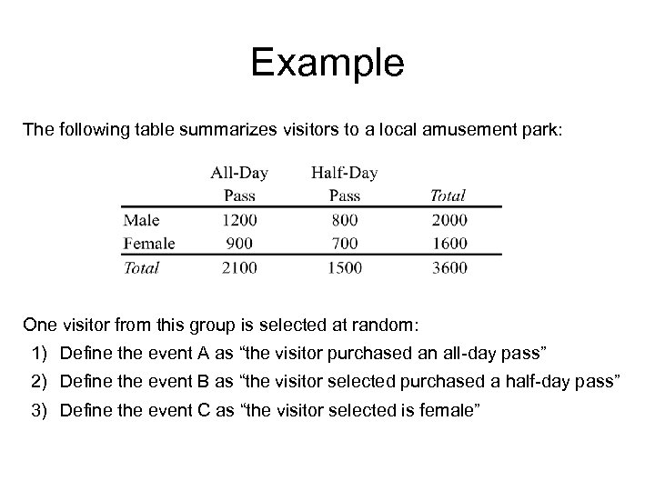
Example The following table summarizes visitors to a local amusement park: One visitor from this group is selected at random: 1) Define the event A as “the visitor purchased an all-day pass” 2) Define the event B as “the visitor selected purchased a half-day pass” 3) Define the event C as “the visitor selected is female”
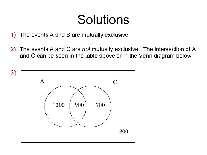
Solutions 1) The events A and B are mutually exclusive 2) The events A and C are not mutually exclusive. The intersection of A and C can be seen in the table above or in the Venn diagram below: 3)
Addition Rule for Disjoint Events • For disjoint events, the outcomes of (E or F) can be listed as the outcomes of E followed by the outcomes of F • There are no duplicates in this list • The Addition Rule for disjoint events is P(E or F) = P(E) + P(F) • Thus we can find P(E or F) if we know both P(E) and P(F)
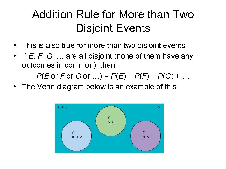
Addition Rule for More than Two Disjoint Events • This is also true for more than two disjoint events • If E, F, G, … are all disjoint (none of them have any outcomes in common), then P(E or F or G or …) = P(E) + P(F) + P(G) + … • The Venn diagram below is an example of this
Example • In rolling a fair die, what is the chance of rolling a {2 or lower} or a {6} – The probability of {2 or lower} is 2/6 – The probability of {6} is 1/6 – The two events {1, 2} and {6} are disjoint • The total probability is 2/6 + 1/6 = 3/6 = 1/2
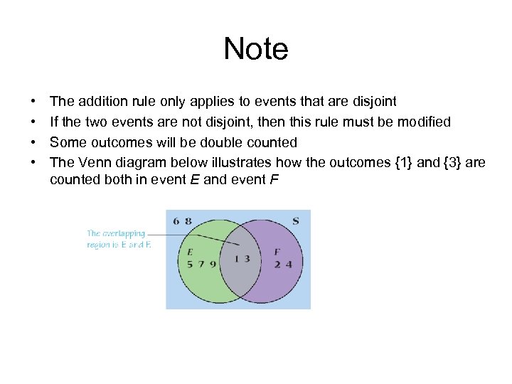
Note • • The addition rule only applies to events that are disjoint If the two events are not disjoint, then this rule must be modified Some outcomes will be double counted The Venn diagram below illustrates how the outcomes {1} and {3} are counted both in event E and event F
Example In rolling a fair die, what is the chance of rolling a {2 or lower} or an even number? – The probability of {2 or lower} is 2/6 – The probability of {2, 4, 6} is 3/6 – The two events {1, 2} and {2, 4, 6} are not disjoint – The total probability is not 2/6 + 3/6 = 5/6 – The total probability is 4/6 because the event is {1, 2, 4, 6} Note: When we say A or B, we include outcomes either in A or in B or both.
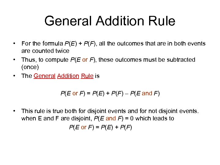
General Addition Rule • For the formula P(E) + P(F), all the outcomes that are in both events are counted twice • Thus, to compute P(E or F), these outcomes must be subtracted (once) • The General Addition Rule is P(E or F) = P(E) + P(F) – P(E and F) • This rule is true both for disjoint events and for not disjoint events. when E and F are disjoint, P(E and F) = 0 which leads to P(E or F) = P(E) + P(F)
Example • When choosing a card at random out of a deck of 52 cards, what is the probability of choosing a queen or a heart? – E = “choosing a queen” – F = “choosing a heart” • E and F are not disjoint (it is possible to choose the queen of hearts), so we must use the General Addition Rule
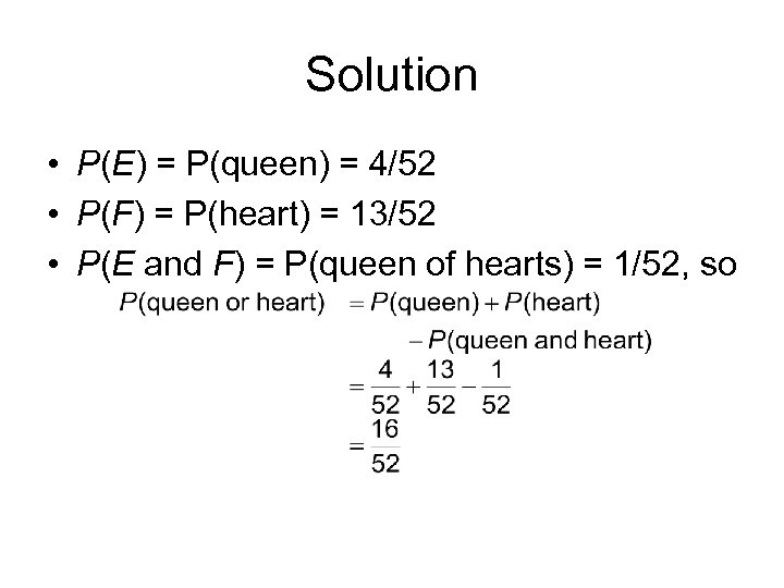
Solution • P(E) = P(queen) = 4/52 • P(F) = P(heart) = 13/52 • P(E and F) = P(queen of hearts) = 1/52, so
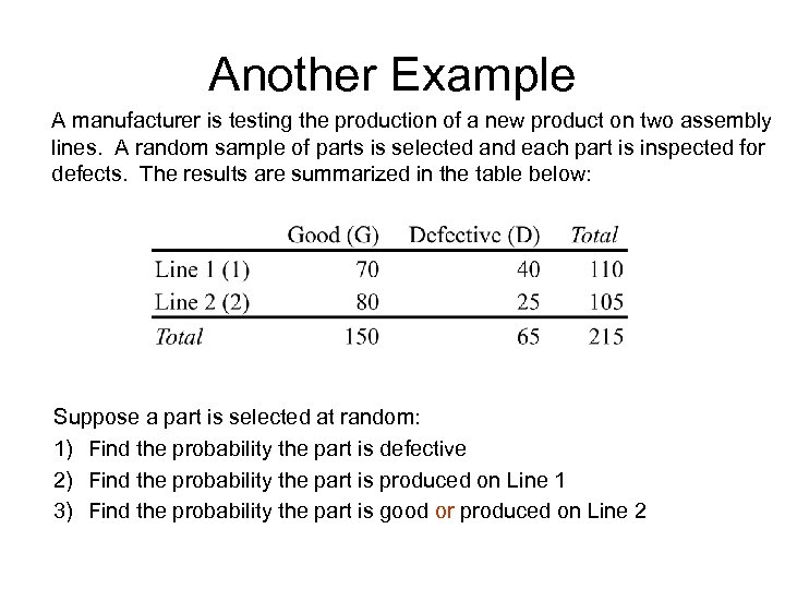
Another Example A manufacturer is testing the production of a new product on two assembly lines. A random sample of parts is selected and each part is inspected for defects. The results are summarized in the table below: Suppose a part is selected at random: 1) Find the probability the part is defective 2) Find the probability the part is produced on Line 1 3) Find the probability the part is good or produced on Line 2
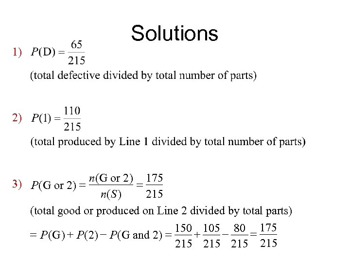
Solutions 1) 2) 3) P (G or 2) = n(G or 2) = 175 n( S ) 215 (total good or produced on Line 2 divided by total parts) 150 105 80 = 175 = P (G ) + P (2) - P (G and 2) = + 215 215
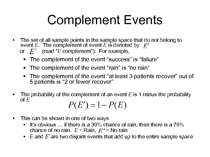
Complement Events • The set of all sample points in the sample space that do not belong to event E. The complement of event E is denoted by or (read “E complement”). For example, § The complement of the event “success” is “failure” § The complement of the event “rain” is “no rain” § The complement of the event “at least 3 patients recover” out of 5 patients is “ 2 or fewer recover” • The probability of the complement of an event E is 1 minus the probability of E • This can be shown in one of two ways § It’s obvious … if there is a 30% chance of rain, then there is a 70% chance of no rain. E = Rain, = No rain § E and are two disjoint events that add up to the entire sample space
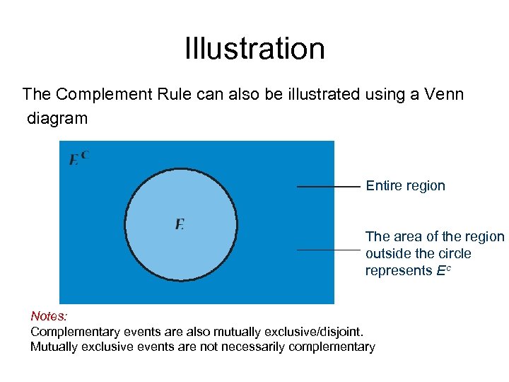
Illustration The Complement Rule can also be illustrated using a Venn diagram Entire region The area of the region outside the circle represents Ec Notes: Complementary events are also mutually exclusive/disjoint. Mutually exclusive events are not necessarily complementary
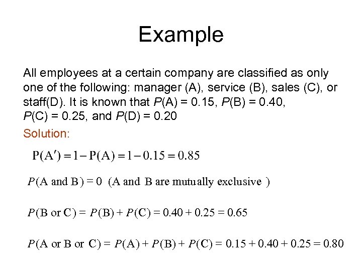
Example All employees at a certain company are classified as only one of the following: manager (A), service (B), sales (C), or staff(D). It is known that P(A) = 0. 15, P(B) = 0. 40, P(C) = 0. 25, and P(D) = 0. 20 Solution: P( A and B ) = 0 (A and B are mutually exclusive ) P ( B or C ) = P ( B) + P ( C ) = 0. 40 + 0. 25 = 0. 65 P ( A or B or C ) = P ( A ) + P ( B) + P ( C ) = 0. 15 + 0. 40 + 0. 25 = 0. 80
Summary • Probabilities obey Additional Rules • For disjoint events, the Addition Rule is used for calculating “or” probabilities • For events that are not disjoint, the Addition Rule is not valid … instead the General Addition Rule is used for calculating “or” probabilities • The Complement Rule is used for calculating “not” probabilities
Independence • Definition of independence: Events E and F are independent if the occurrence of E in a probability experiment does not affect the probability of event F • Other ways of saying the same thing – Knowing E does not give any additional information about F – Knowing F does not give any additional information about E – E and F are totally unrelated
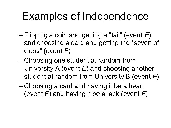
Examples of Independence – Flipping a coin and getting a “tail” (event E) and choosing a card and getting the “seven of clubs” (event F) – Choosing one student at random from University A (event E) and choosing another student at random from University B (event F) – Choosing a card and having it be a heart (event E) and having it be a jack (event F)
Dependent Events • If the two events are not independent, then they are said to be dependent • Dependent does not mean that they completely rely on each other … it just means that they are not independent of each other • Dependent means that there is some kind of relationship between E and F – even if it is just a very small relationship
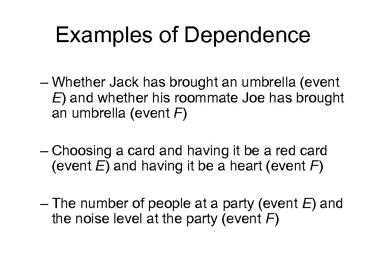
Examples of Dependence – Whether Jack has brought an umbrella (event E) and whether his roommate Joe has brought an umbrella (event F) – Choosing a card and having it be a red card (event E) and having it be a heart (event F) – The number of people at a party (event E) and the noise level at the party (event F)
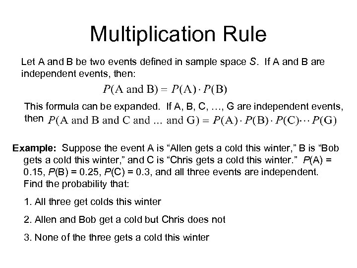
Multiplication Rule Let A and B be two events defined in sample space S. If A and B are independent events, then: This formula can be expanded. If A, B, C, …, G are independent events, then Example: Suppose the event A is “Allen gets a cold this winter, ” B is “Bob gets a cold this winter, ” and C is “Chris gets a cold this winter. ” P(A) = 0. 15, P(B) = 0. 25, P(C) = 0. 3, and all three events are independent. Find the probability that: 1. All three get colds this winter 2. Allen and Bob get a cold but Chris does not 3. None of the three gets a cold this winter
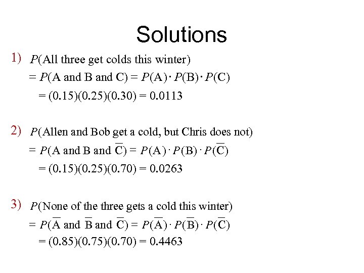
Solutions 1) P(All three get colds this winter ) = P (A and B and C) = P (A ) × P( B) × P (C) = (0. 15)(0. 25)(0. 30) = 0. 0113 2) P ( Allen and Bob get a cold, but Chris does not) = P ( A and B and C ) = P ( A ) × P ( B) × P ( C ) = (0. 15)(0. 25)(0. 70) = 0. 0263 3) P ( None of the three gets a cold this winter) = P ( A and B and C ) = P ( A ) × P ( B) × P ( C) = (0. 85)(0. 70) = 0. 4463
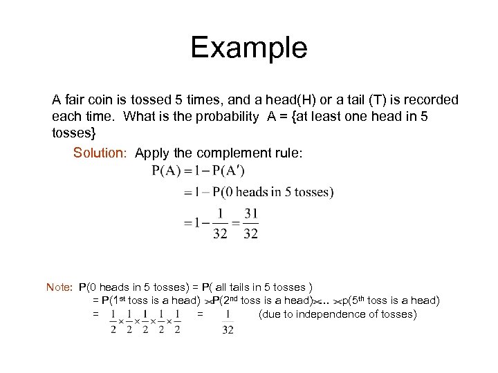
Example A fair coin is tossed 5 times, and a head(H) or a tail (T) is recorded each time. What is the probability A = {at least one head in 5 tosses} Solution: Apply the complement rule: Note: P(0 heads in 5 tosses) = P( all tails in 5 tosses ) = P(1 st toss is a head) P(2 nd toss is a head) … p(5 th toss is a head) = = (due to independence of tosses)
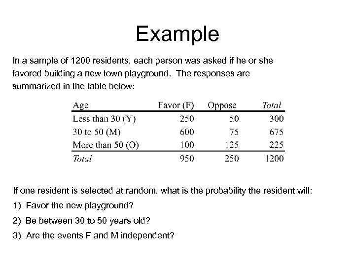
Example In a sample of 1200 residents, each person was asked if he or she favored building a new town playground. The responses are summarized in the table below: If one resident is selected at random, what is the probability the resident will: 1) Favor the new playground? 2) Be between 30 to 50 years old? 3) Are the events F and M independent?
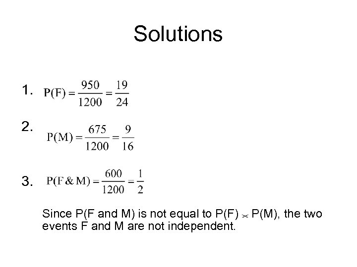
Solutions 1. 2. 3. Since P(F and M) is not equal to P(F) events F and M are not independent. P(M), the two
Mutually Exclusive Events Are Not Independent • What’s the difference between disjoint events and independent events? • Disjoint events can never be independent – – Consider two events E and F that are disjoint Let’s say that event E has occurred Then we know that event F cannot have occurred Knowing information about event E has told us much information about event F – Thus E and F are not independent
Summary • Compound Events are formed by combining several simple events: § The probability that either event A or event B will occur: P(A or B) § The probability that both events A and B will occur: P(A and B) • The “disjoint” concept corresponds to “or” and the Addition Rule … disjoint events and adding probabilities • The concept of independence corresponds to “and” and the Multiplication Rule … independent events and multiplying probabilities
Discrete Probability Distributions Discrete Random Variables, Discrete Probability Distribution The Binomial Probability Distribution
Learning Objectives 1. Distinguish between discrete and continuous random variables 2. Identify discrete probability distributions 3. Construct probability histograms 4. Compute and interpret the mean of a discrete random variable 5. Interpret the mean of a discrete random variable as an expected value 6. Compute the variance and standard deviation of a discrete random variable
Discrete Random Variable
Random Variables If the outcomes from an experiment are quantitative type (i. e. numbers), we denote the outcomes of this type with a variable using a capital letter such as X, Y , Z … That is, the variable contains all possible values (i. e. outcomes) from the experiment. Each possible value is denoted with lower case letter such as x, y, z… Since there is a probability/chance for each value of the variable to occur, we call the variable as a random variable.
Examples of Random Variables • Tossing four coins and counting the number of heads – The number could be 0, 1, 2, 3, or 4 – The number could change when we toss another four coins • Measuring the heights of students - The heights could vary from student to student • Recording the number of computers sold per day by a local merchant with a random variable. Integer values ranging from zero to about 50 are possible values.
Discrete Random Variables • A discrete random variable is a random variable that has either a finite or a countable number of values – A finite number of values such as {0, 1, 2, 3, and 4} – A countable number of values such as {1, 2, 3, …} • Discrete random variables are often “counts of …”
Examples of Discrete Random Variables • The number of heads in tossing 3 coins There are four possible values – 0 heads, 1 head, 2 heads, and 3 heads – A finite number of possible values – a discrete random variable – This fits our general concept that discrete random variables are often “counts of …” • The number of pages in statistics textbooks – A countable number of possible values • The number of visitors to the White House in a day – A countable number of possible values
Continuous Random Variables • A continuous random variable is a random variable that has an infinite, and more than countable, number of values – The values are any number in an interval • Continuous random variables are often “measurements of …”
Examples of Continuous Random Variables • The possible temperature in Chicago at noon tomorrow, measured in degrees Fahrenheit – The possible values (assuming that we can measure temperature to great accuracy) are in an interval. So, 20 degrees can be recorded as 20. 4 degrees or 20. 41 degrees … etc. – The interval may be something like from -20 to 110 degrees. – This fits our general concept that continuous random variables are often “measurements of …” • The height of a college student – A value in an interval between 3 and 8 feet • The number of bytes of storage used on a 80 GB (80 billion bytes) hard drive – Although this is discrete, it is more reasonable to model it as a continuous random variable between 0 and 80 GB
Discrete Probability Distribution
Probability Distribution • Probability Distribution is a distribution of the probabilities associated with each of the values of a random variable. • The probability distribution is a theoretical distribution because the probabilities are theoretical probabilities; it is used to represent populations.
Discrete Probability Distribution • The probability distribution of a discrete random variable X relates the values of X with their corresponding probabilities • A distribution could be – In the form of a table – In the form of a graph – In the form of a mathematical formula
Probability Function • If X is a discrete random variable and x is a possible value for X, then we write P(x) as the probability that X is equal to x • Examples – In tossing one coin, if X is the number of heads, then P(0) = 0. 5 and P(1) = 0. 5 – In rolling one die, if X is the number rolled, then P(1) = 1/6
Properties of P(x) • Since P(x) form a probability distribution, they must satisfy the rules of probability – 0 ≤ P(x) ≤ 1 – Σ P(x) = 1 • In the second rule, the Σ sign means to add up the P(x)’s for all the possible x’s
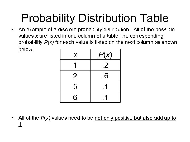
Probability Distribution Table • An example of a discrete probability distribution. All of the possible values x are listed in one column of a table, the corresponding probability P(x) for each value is listed on the next column as shown below: x 1 2 5 6 P(x). 2. 6. 1. 1 • All of the P(x) values need to be not only positive but also add up to 1
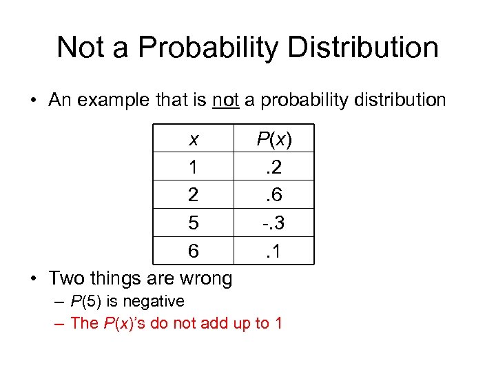
Not a Probability Distribution • An example that is not a probability distribution x 1 2 5 6 • Two things are wrong P(x). 2. 6 -. 3. 1 – P(5) is negative – The P(x)’s do not add up to 1
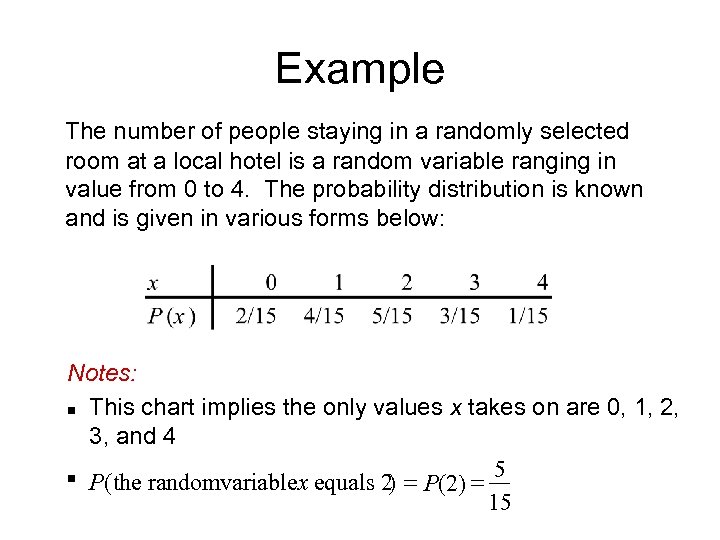
Example The number of people staying in a randomly selected room at a local hotel is a random variable ranging in value from 0 to 4. The probability distribution is known and is given in various forms below: Notes: n This chart implies the only values x takes on are 0, 1, 2, 3, and 4 5 n P( the randomvariablex equals 2 = P(2) = ) 15
Probability Histogram • A probability histogram is a histogram where – The horizontal axis corresponds to the possible values of X (i. e. the x’s) – The vertical axis corresponds to the probabilities for those values (i. e. the P(x)’s) • A probability histogram is very similar to a relative frequency histogram
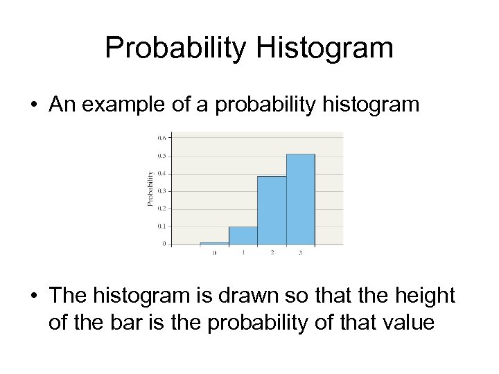
Probability Histogram • An example of a probability histogram • The histogram is drawn so that the height of the bar is the probability of that value
Notes • The histogram of a probability distribution uses the area of each bar to represent its assigned probability • The width of each bar is 1 and the height of each bar is the assigned probability, so the area of each bar is also equal to the corresponding probability • The idea of area representing probability is important in the study of continuous random variables later
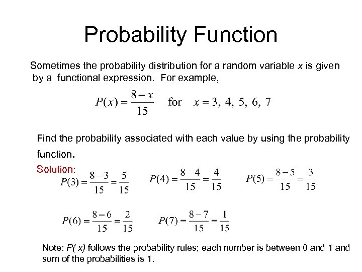
Probability Function Sometimes the probability distribution for a random variable x is given by a functional expression. For example, Find the probability associated with each value by using the probability function. Solution: Note: P( x) follows the probability rules; each number is between 0 and 1 and sum of the probabilities is 1.
Mean of Probability Distribution • Probability distribution is a population distribution, because the probability is regarded as an idealized relative frequency for an outcome to occur if the experiment is repeated large number of times (mostly infinite times if we can). • Since the mean of a population is denoted by a parameter m, the mean of a probability distribution is denoted by m as well • The mean of a probability distribution can be thought of in this way: – There are various possible values of a discrete random variable – The values that have the higher probabilities are the ones that occur more often – The values that occur more often should have a larger role in calculating the mean – The mean of the probability distribution is the weighted average of the values, weighted by the probabilities
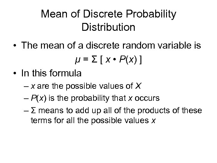
Mean of Discrete Probability Distribution • The mean of a discrete random variable is μ = Σ [ x • P(x) ] • In this formula – x are the possible values of X – P(x) is the probability that x occurs – Σ means to add up all of the products of these terms for all the possible values x
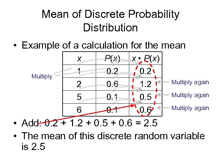
Mean of Discrete Probability Distribution • Example of a calculation for the mean P(x) 0. 2 0. 6 x • P(x) 0. 2 1. 2 5 6 Multiply x 1 2 0. 1 0. 5 0. 6 Multiply again • Add: 0. 2 + 1. 2 + 0. 5 + 0. 6 = 2. 5 • The mean of this discrete random variable is 2. 5
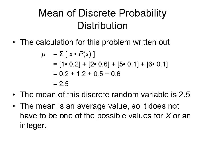
Mean of Discrete Probability Distribution • The calculation for this problem written out μ = Σ [ x • P(x) ] = [1 • 0. 2] + [2 • 0. 6] + [5 • 0. 1] + [6 • 0. 1] = 0. 2 + 1. 2 + 0. 5 + 0. 6 = 2. 5 • The mean of this discrete random variable is 2. 5 • The mean is an average value, so it does not have to be one of the possible values for X or an integer.
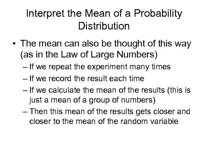
Interpret the Mean of a Probability Distribution • The mean can also be thought of this way (as in the Law of Large Numbers) – If we repeat the experiment many times – If we record the result each time – If we calculate the mean of the results (this is just a mean of a group of numbers) – Then this mean of the results gets closer and closer to the mean of the random variable
Expected Value • The expected value of a random variable is another term for its mean. That is, we often interpret the mean of a discrete random variable as an expected value • The term “expected value” illustrates the long term nature of the experiments as described on the previous slide – as we perform more and more experiments, the mean of the results of those experiments gets closer to the “expected value” of the random variable
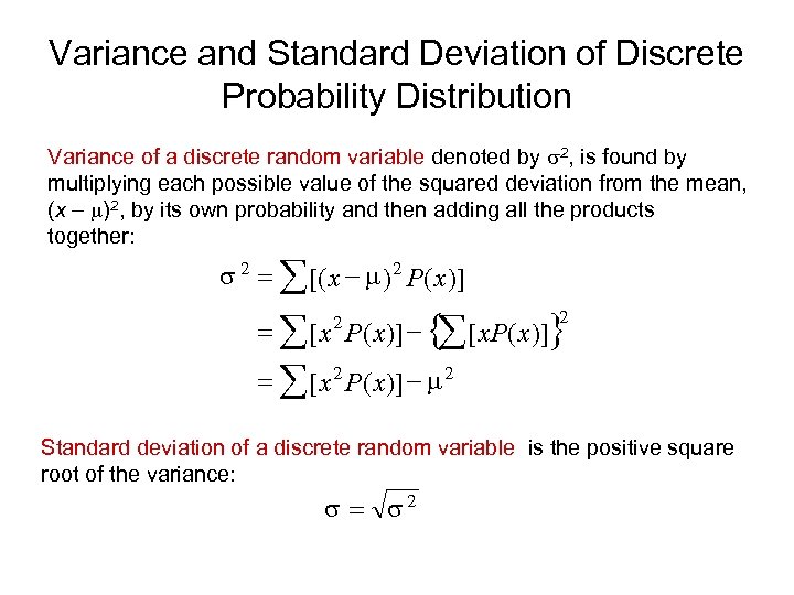
Variance and Standard Deviation of Discrete Probability Distribution Variance of a discrete random variable denoted by s 2, is found by multiplying each possible value of the squared deviation from the mean, (x - m)2, by its own probability and then adding all the products together: s 2 = å [( x - m ) 2 P ( x )] = å [ x 2 P ( x )] - { [ x. P ( x )]} å 2 = å [ x 2 P ( x )] - m 2 Standard deviation of a discrete random variable is the positive square root of the variance: s = s 2
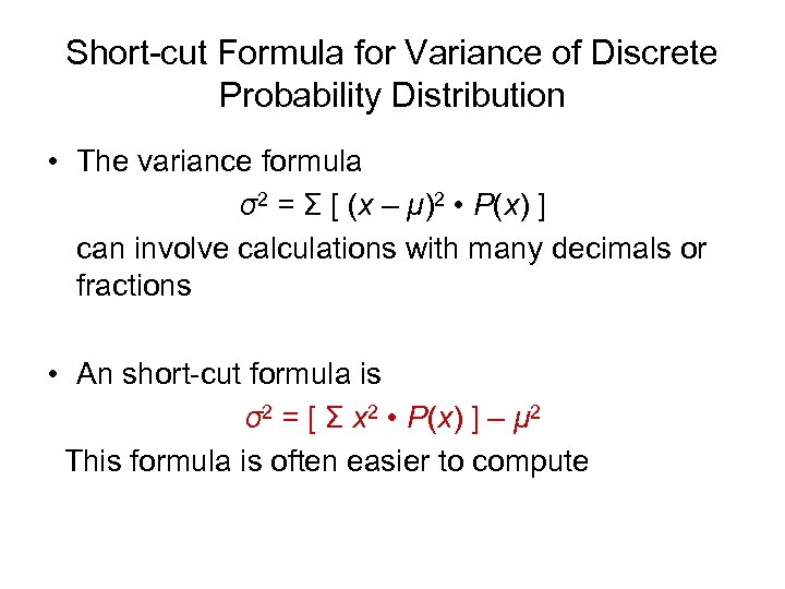
Short-cut Formula for Variance of Discrete Probability Distribution • The variance formula σ2 = Σ [ (x – μ)2 • P(x) ] can involve calculations with many decimals or fractions • An short-cut formula is σ2 = [ Σ x 2 • P(x) ] – μ 2 This formula is often easier to compute
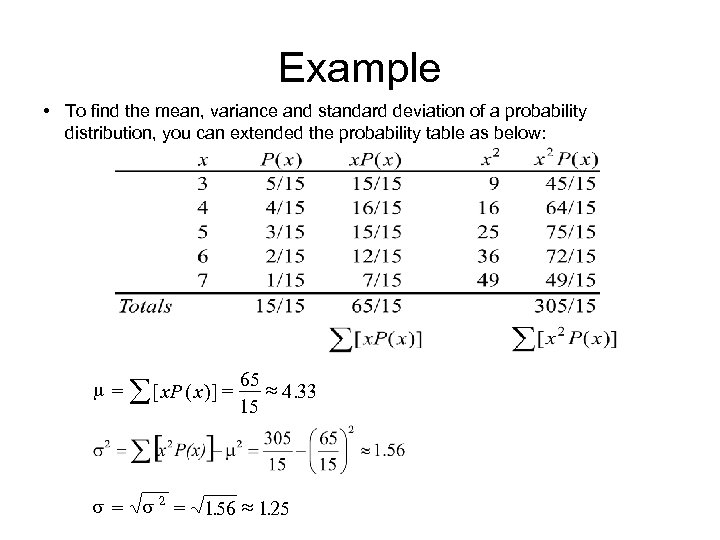
Example • To find the mean, variance and standard deviation of a probability distribution, you can extended the probability table as below: m= å [ x. P ( x )] = 65 » 4. 33 15 s = s 2 = 1. 56 » 1. 25
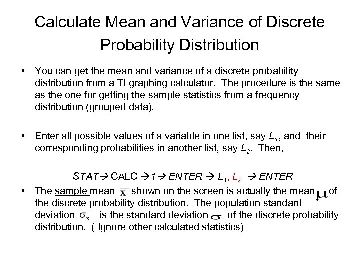
Calculate Mean and Variance of Discrete Probability Distribution • You can get the mean and variance of a discrete probability distribution from a TI graphing calculator. The procedure is the same as the one for getting the sample statistics from a frequency distribution (grouped data). • Enter all possible values of a variable in one list, say L 1, and their corresponding probabilities in another list, say L 2. Then, STAT CALC 1 ENTER L 1, L 2 ENTER • The sample mean shown on the screen is actually the mean of the discrete probability distribution. The population standard deviation is the standard deviation of the discrete probability distribution. ( Ignore other calculated statistics)
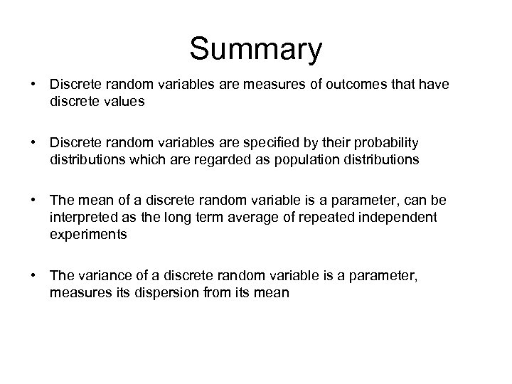
Summary • Discrete random variables are measures of outcomes that have discrete values • Discrete random variables are specified by their probability distributions which are regarded as population distributions • The mean of a discrete random variable is a parameter, can be interpreted as the long term average of repeated independent experiments • The variance of a discrete random variable is a parameter, measures its dispersion from its mean
The Binomial Probability Distribution
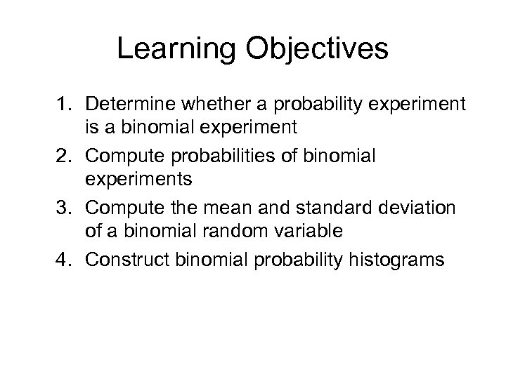
Learning Objectives 1. Determine whether a probability experiment is a binomial experiment 2. Compute probabilities of binomial experiments 3. Compute the mean and standard deviation of a binomial random variable 4. Construct binomial probability histograms
Binomial Experiment • A binomial experiment has the following structure – The first trial of the experiment is performed … the result is either a success or a failure (Outcomes are classified into two categories, so it is term binomial experiment. ) – The second trial is performed … the result is either a success or a failure. This result is independent of the first and the chance of success is the same as the first trial. – A third trial is performed … the result is either a success or a failure. The result is independent of the first two and the chance of success is the same – The process can go on and on.
Example – A card is drawn from a deck. A “success” is for that card to be a heart … a “failure” is for any other suit – The card is then put back into the deck – A second card is drawn from the deck with the same definition of success. – The second card is put back into the deck – We continue for drawing 10 cards
Binomial Experiment A binomial experiment is an experiment with the following characteristics – The experiment is performed a fixed number of times, each time called a trial – The trials are independently performed – Each trial has two possible outcomes, usually called a success (desired outcomes) and a failure (the rest of other outcomes) – The probability of success is the same for every trial Note: If an experiment contains more than 2 outcomes. We can always classify the outcome into two categories, success and failure. For instance, tossing a die, success is having a number less than 3, then failure is having a number not less than 3.
Binomial Probability Distribution • Notation used for binomial distributions – The number of trials is represented by n – The probability of a success is represented by p – The total number of successes in n trials is the ransom variable X, the outcome observed • Because there cannot be a negative number of successes, and because there cannot be more than n successes (out of n attempts) 0≤X≤n
Example • In our card drawing example – Each trial is the experiment of drawing one card – The experiment is performed 10 times, so n = 10 – The trials are independent because the drawn card is put back into the deck so that a card drawn before will not affect a card drawn next. – Each trial has two possible outcomes, a “success” of drawing a heart and a “failure” of drawing anything else – The probability of success is 0. 25 (Since there are four suits in a deck where heart is one of the suits), the same for every trial, so p = 0. 25 – X, the number of successes, is between 0 and 10
Notes • The word “success” does not mean that this is a good outcome or that we want this to be the outcome • A “success” in our card drawing experiment is to draw a heart • If we are counting hearts, then this is the outcome that we are measuring • There is no good or bad meaning to “success”
Calculate Binomial Probability • We would like to calculate the probabilities of X, i. e. P(0), P(1), P(2), …, P(n) • Do a simpler example first – For n = 3 trials (e. g. toss a coin 3 time) – With p =. 4 probability of success (e. g. Head is a success. The coin is loaded such that P(head) = 0. 4) – Calculate P(2), the probability of 2 successes (i. e. 2 heads)
Calculate Binomial Probability • For 3 trials, the possible ways of getting exactly 2 successes are –S S F –S F S –F S S • The probabilities for each (using the multiplication rule of independent events) are – 0. 4 • 0. 6 = 0. 096 – 0. 4 • 0. 6 • 0. 4 = 0. 096 – 0. 6 • 0. 4 = 0. 096
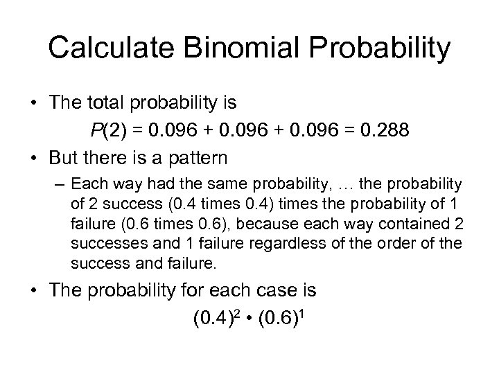
Calculate Binomial Probability • The total probability is P(2) = 0. 096 + 0. 096 = 0. 288 • But there is a pattern – Each way had the same probability, … the probability of 2 success (0. 4 times 0. 4) times the probability of 1 failure (0. 6 times 0. 6), because each way contained 2 successes and 1 failure regardless of the order of the success and failure. • The probability for each case is (0. 4)2 • (0. 6)1
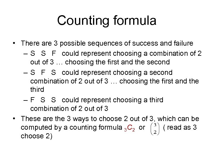
Counting formula • There are 3 possible sequences of success and failure – S S F could represent choosing a combination of 2 out of 3 … choosing the first and the second – S F S could represent choosing a second combination of 2 out of 3 … choosing the first and the third – F S S could represent choosing a third combination of 2 out of 3 • These are the 3 ways to choose 2 out of 3, which can be computed by a counting formula 3 C 2 or ( read as 3 choose 2)
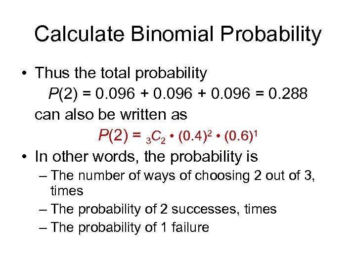
Calculate Binomial Probability • Thus the total probability P(2) = 0. 096 + 0. 096 = 0. 288 can also be written as P(2) = 3 C 2 • (0. 4)2 • (0. 6)1 • In other words, the probability is – The number of ways of choosing 2 out of 3, times – The probability of 2 successes, times – The probability of 1 failure
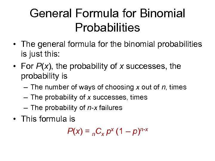
General Formula for Binomial Probabilities • The general formula for the binomial probabilities is just this: • For P(x), the probability of x successes, the probability is – The number of ways of choosing x out of n, times – The probability of x successes, times – The probability of n-x failures • This formula is P(x) = n. Cx px (1 – p)n-x
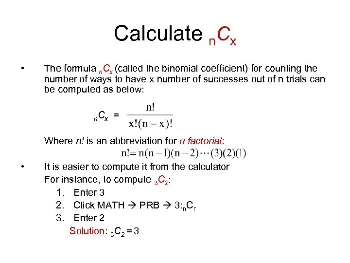
Calculate n. Cx • The formula n. Cx (called the binomial coefficient) for counting the number of ways to have x number of successes out of n trials can be computed as below: n Cx = Where n! is an abbreviation for n factorial: • It is easier to compute it from the calculator For instance, to compute 3 C 2: 1. Enter 3 2. Click MATH PRB 3: n. Cr 3. Enter 2 Solution: 3 C 2 = 3
Example • A student guesses at random on a multiple choice quiz – There are n = 10 questions in total – There are 5 choices per question so that the probability of success (guess correctly) p = 1/5 =. 2 (due to random guessing, each choice has equal chance) • What is the probability that the student gets 6 questions correct?
Example Continued First, check if this is a binomial experiment – There a finite number n = 10 of trials (10 questions, answer one question each trial) – Each trial has two outcomes (a correct guess and an incorrect guess) – The probability of success is independent from trial to trial (every question is done by a random guess) – The probability of success p =. 2 is the same for each trial
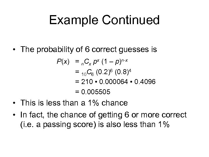
Example Continued • The probability of 6 correct guesses is P(x) = n. Cx px (1 – p)n-x = 10 C 6 (0. 2)6 (0. 8)4 = 210 • 0. 000064 • 0. 4096 = 0. 005505 • This is less than a 1% chance • In fact, the chance of getting 6 or more correct (i. e. a passing score) is also less than 1%
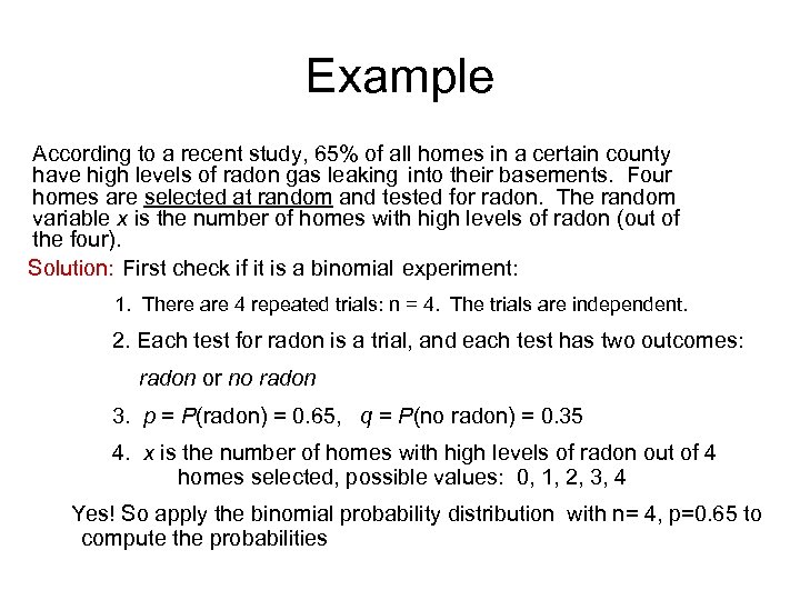
Example According to a recent study, 65% of all homes in a certain county have high levels of radon gas leaking into their basements. Four homes are selected at random and tested for radon. The random variable x is the number of homes with high levels of radon (out of the four). Solution: First check if it is a binomial experiment: 1. There are 4 repeated trials: n = 4. The trials are independent. 2. Each test for radon is a trial, and each test has two outcomes: radon or no radon 3. p = P(radon) = 0. 65, q = P(no radon) = 0. 35 4. x is the number of homes with high levels of radon out of 4 homes selected, possible values: 0, 1, 2, 3, 4 Yes! So apply the binomial probability distribution with n= 4, p=0. 65 to compute the probabilities
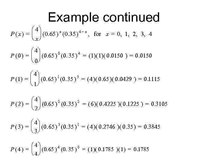
Example continued æ 4ö = ç ÷ (0. 65 ) x (0. 35 ) 4 - x , for x = 0, 1, 2, 3, 4 P( x) è xø æ 4ö 0 4 P ( 0 ) = ç ÷ (0. 65 ) (0. 35 ) = (1)( 0. 0150 ) = 0. 0150 è 0ø æ 4ö = ç ÷ (0. 65 ) 1 (0. 35 ) 3 = ( 4 )( 0. 65 )( 0. 0429 ) = 0. 1115 P (1) è 1ø æ 4ö = ç ÷ (0. 65 ) 2 (0. 35 ) 2 = ( 6 )( 0. 4225 )( 0. 1225 ) = 0. 3105 P (2) è 2ø æ 4ö = ç ÷ (0. 65 ) 3 (0. 35 ) 1 = ( 4 )( 0. 2746 )( 0. 35 ) = 0. 3845 P ( 3) è 3ø æ 4ö = ç ÷ (0. 65 ) 4 (0. 35 ) 0 = ( 1)( 0. 1785 )( 1) = 0. 1785 P (4) è 4ø
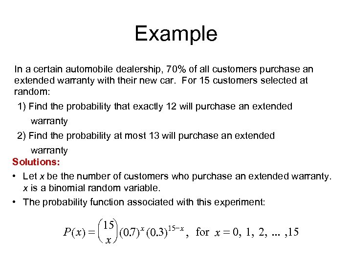
Example In a certain automobile dealership, 70% of all customers purchase an extended warranty with their new car. For 15 customers selected at random: 1) Find the probability that exactly 12 will purchase an extended warranty 2) Find the probability at most 13 will purchase an extended warranty Solutions: • Let x be the number of customers who purchase an extended warranty. x is a binomial random variable. • The probability function associated with this experiment: æ 15ö P ( x ) = ç ÷ (0. 7) x (0. 3)15 - x , for x = 0, 1, 2, . . . , 15 è xø
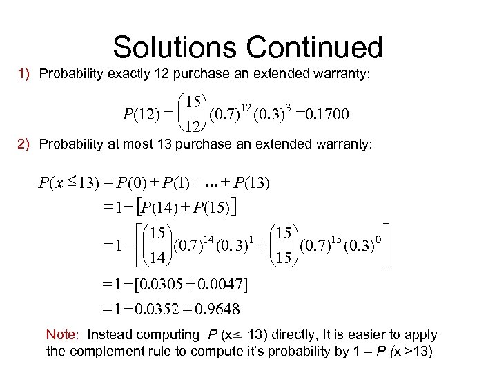
Solutions Continued 1) Probability exactly 12 purchase an extended warranty: æ 15ö P(12) = ç ÷ (0. 7)12 (0. 3) 3 =0. 1700 è 12ø 2) Probability at most 13 purchase an extended warranty: P ( x £ 13) = P (0) + P (1) +. . . + P (13) = 1 - [P (14) + P (15)] éæ 15 ö 14 1 æ 15 ö 15 0ù = 1 - êç ÷(0. 7) (0. 3) + ç ÷(0. 7) (0. 3) ú è 15 ø ëè 14 ø û = 1 - [0. 0305 + 0. 0047] = 1 - 0. 0352 = 0. 9648 Note: Instead computing P (x 13) directly, It is easier to apply the complement rule to compute it’s probability by 1 – P (x >13)
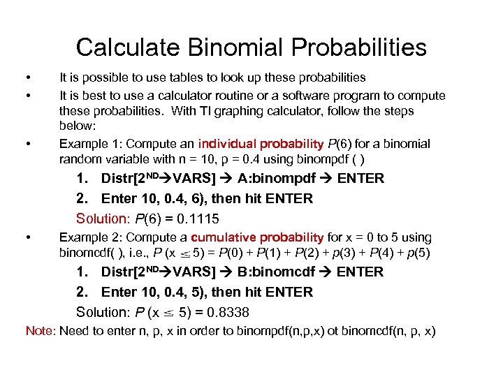
Calculate Binomial Probabilities • • • It is possible to use tables to look up these probabilities It is best to use a calculator routine or a software program to compute these probabilities. With TI graphing calculator, follow the steps below: Example 1: Compute an individual probability P(6) for a binomial random variable with n = 10, p = 0. 4 using binompdf ( ) 1. Distr[2 ND VARS] A: binompdf ENTER 2. Enter 10, 0. 4, 6), then hit ENTER Solution: P(6) = 0. 1115 • Example 2: Compute a cumulative probability for x = 0 to 5 using binomcdf( ), i. e. , P (x 5) = P(0) + P(1) + P(2) + p(3) + P(4) + p(5) 1. Distr[2 ND VARS] B: binomcdf ENTER 2. Enter 10, 0. 4, 5), then hit ENTER Solution: P (x 5) = 0. 8338 Note: Need to enter n, p, x in order to binompdf(n, p, x) ot binomcdf(n, p, x)
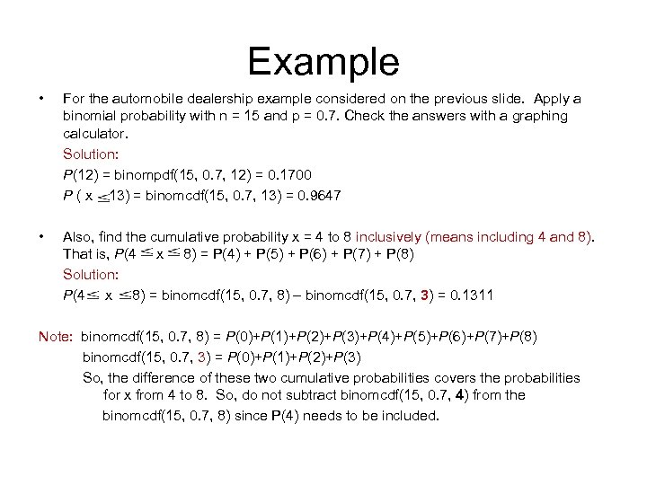
Example • For the automobile dealership example considered on the previous slide. Apply a binomial probability with n = 15 and p = 0. 7. Check the answers with a graphing calculator. Solution: P(12) = binompdf(15, 0. 7, 12) = 0. 1700 P ( x 13) = binomcdf(15, 0. 7, 13) = 0. 9647 • Also, find the cumulative probability x = 4 to 8 inclusively (means including 4 and 8). That is, P(4 x 8) = P(4) + P(5) + P(6) + P(7) + P(8) Solution: P(4 x 8) = binomcdf(15, 0. 7, 8) – binomcdf(15, 0. 7, 3) = 0. 1311 Note: binomcdf(15, 0. 7, 8) = P(0)+P(1)+P(2)+P(3)+P(4)+P(5)+P(6)+P(7)+P(8) binomcdf(15, 0. 7, 3) = P(0)+P(1)+P(2)+P(3) So, the difference of these two cumulative probabilities covers the probabilities for x from 4 to 8. So, do not subtract binomcdf(15, 0. 7, 4) from the binomcdf(15, 0. 7, 8) since P(4) needs to be included.
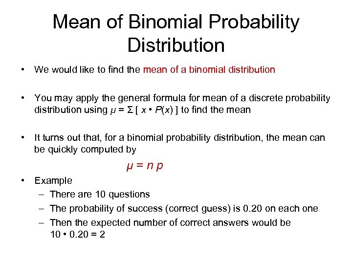
Mean of Binomial Probability Distribution • We would like to find the mean of a binomial distribution • You may apply the general formula for mean of a discrete probability distribution using μ = Σ [ x • P(x) ] to find the mean • It turns out that, for a binomial probability distribution, the mean can be quickly computed by μ=np • Example – There are 10 questions – The probability of success (correct guess) is 0. 20 on each one – Then the expected number of correct answers would be 10 • 0. 20 = 2
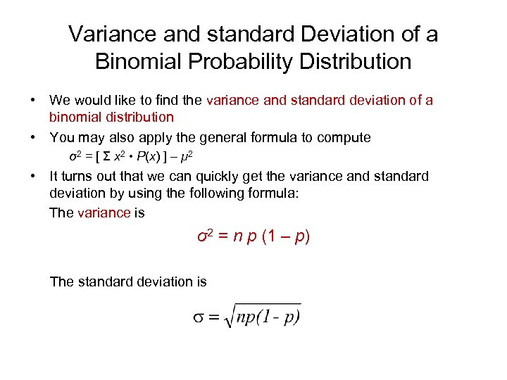
Variance and standard Deviation of a Binomial Probability Distribution • We would like to find the variance and standard deviation of a binomial distribution • You may also apply the general formula to compute σ2 = [ Σ x 2 • P(x) ] – μ 2 • It turns out that we can quickly get the variance and standard deviation by using the following formula: The variance is σ2 = n p (1 – p) The standard deviation is
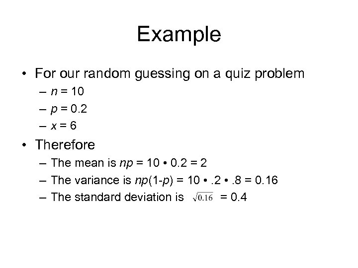
Example • For our random guessing on a quiz problem – n = 10 – p = 0. 2 – x=6 • Therefore – The mean is np = 10 • 0. 2 = 2 – The variance is np(1 -p) = 10 • . 2 • . 8 = 0. 16 – The standard deviation is = 0. 4
Shape of Binomial Distribution • With the formula for the binomial probabilities P(x), we can construct histograms for the binomial distribution • There are three different shapes for these histograms – When p <. 5, the histogram is skewed right – When p =. 5, the histogram is symmetric – When p >. 5, the histogram is skewed left
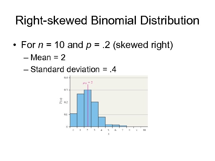
Right-skewed Binomial Distribution • For n = 10 and p =. 2 (skewed right) – Mean = 2 – Standard deviation =. 4
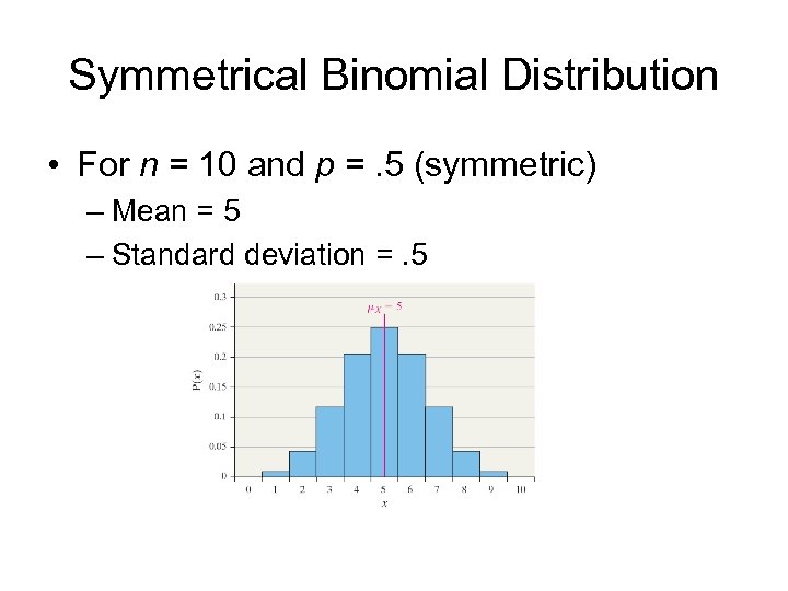
Symmetrical Binomial Distribution • For n = 10 and p =. 5 (symmetric) – Mean = 5 – Standard deviation =. 5
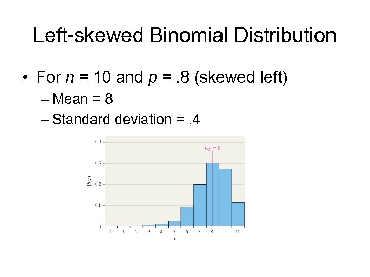
Left-skewed Binomial Distribution • For n = 10 and p =. 8 (skewed left) – Mean = 8 – Standard deviation =. 4
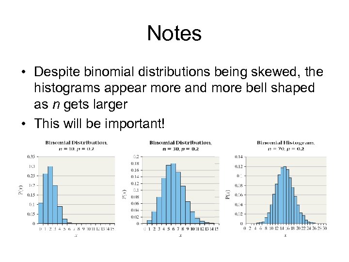
Notes • Despite binomial distributions being skewed, the histograms appear more and more bell shaped as n gets larger • This will be important!
Summary • Binomial random variables model a series of independent trials, each of which can be a success or a failure, each of which has the same probability of success • The binomial random variable has mean equal to np and variance equal to np(1 -p)
3f5c3f93a19e684d37579f71ad9395a8.ppt