Pricing Strategy Example of Profit Maximization

Pricing Strategy

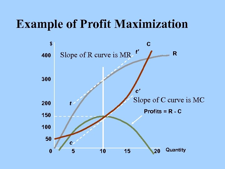Example of Profit Maximization $ 400 C Slope of R curve is MR t' R 300 c’ 200 Slope of C curve is MC t Profits = R - C 150 100 50 0 c 5 10 15 20 Quantity

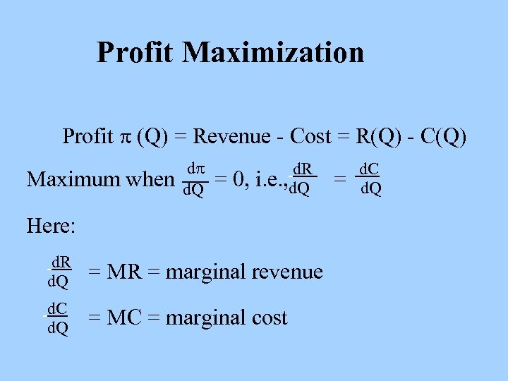Profit Maximization Profit (Q) = Revenue - Cost = R(Q) - C(Q) Maximum when d d. Q = 0, d. R i. e. , d. Q Here: d. R d. Q = MR = marginal revenue d. C d. Q = MC = marginal cost = d. C d. Q

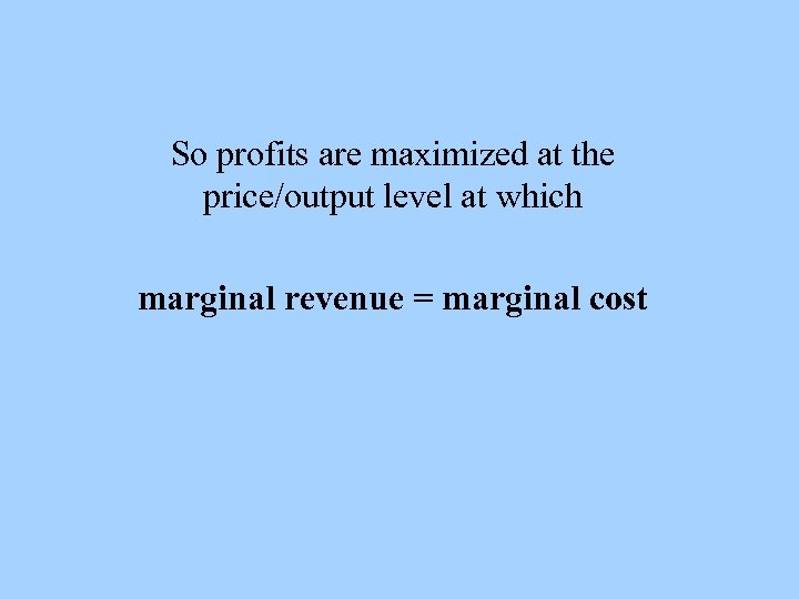So profits are maximized at the price/output level at which marginal revenue = marginal cost

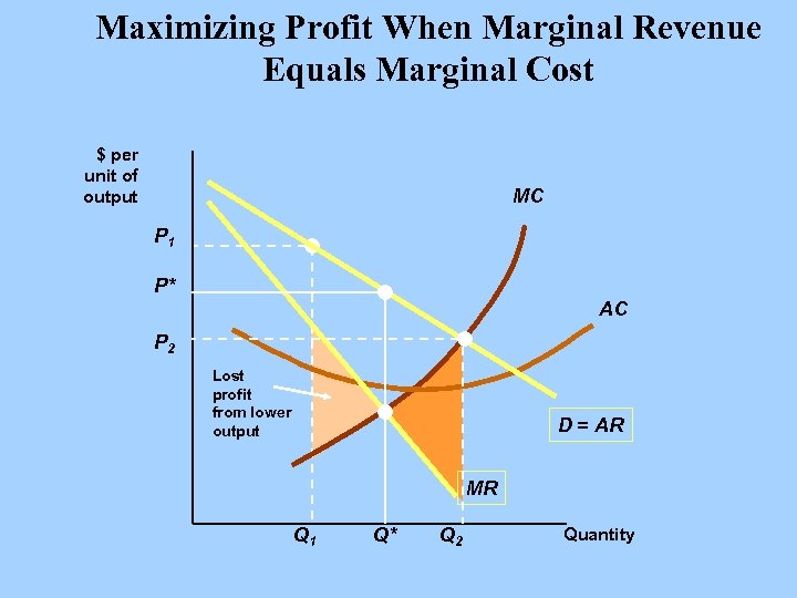Maximizing Profit When Marginal Revenue Equals Marginal Cost $ per unit of output MC P 1 P* AC P 2 Lost profit from lower output D = AR MR Q 1 Q* Q 2 Quantity

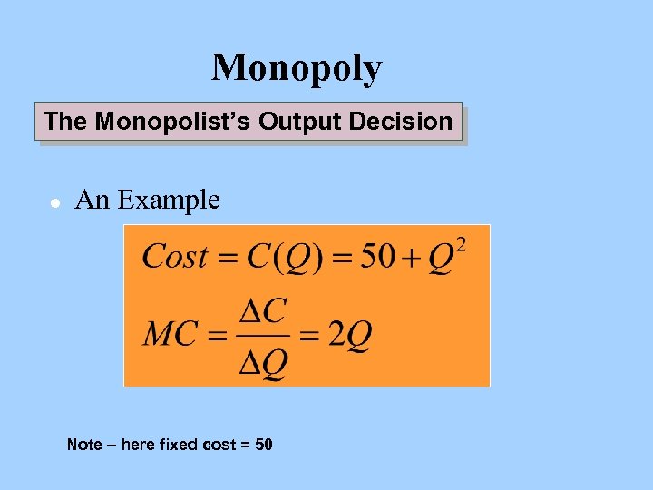Monopoly The Monopolist’s Output Decision l An Example Note – here fixed cost = 50

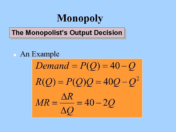Monopoly The Monopolist’s Output Decision l An Example

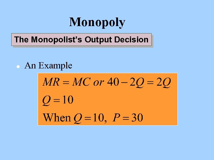Monopoly The Monopolist’s Output Decision l An Example

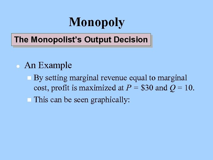Monopoly The Monopolist’s Output Decision l An Example By setting marginal revenue equal to marginal cost, profit is maximized at P = $30 and Q = 10. n This can be seen graphically: n

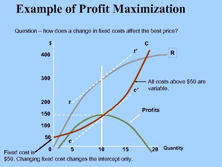Example of Profit Maximization Question – how does a change in fixed costs affect the best price? $ C t' 400 300 c’ 200 R All costs above $50 are variable. t Profits 150 100 50 0 c 5 10 15 Fixed cost is $50. Changing fixed cost changes the intercept only. 20 Quantity

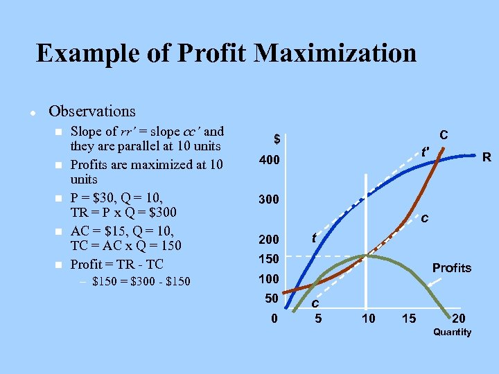Example of Profit Maximization l Observations n n n Slope of rr’ = slope cc’ and they are parallel at 10 units Profits are maximized at 10 units P = $30, Q = 10, TR = P x Q = $300 AC = $15, Q = 10, TC = AC x Q = 150 Profit = TR - TC – $150 = $300 - $150 C $ t' 400 R 300 c 200 t 150 Profits 100 50 c 0 5 10 15 20 Quantity

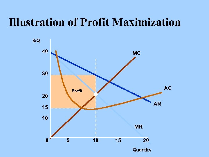Illustration of Profit Maximization $/Q 40 MC 30 AC Profit 20 AR 15 10 MR 0 5 10 15 20 Quantity

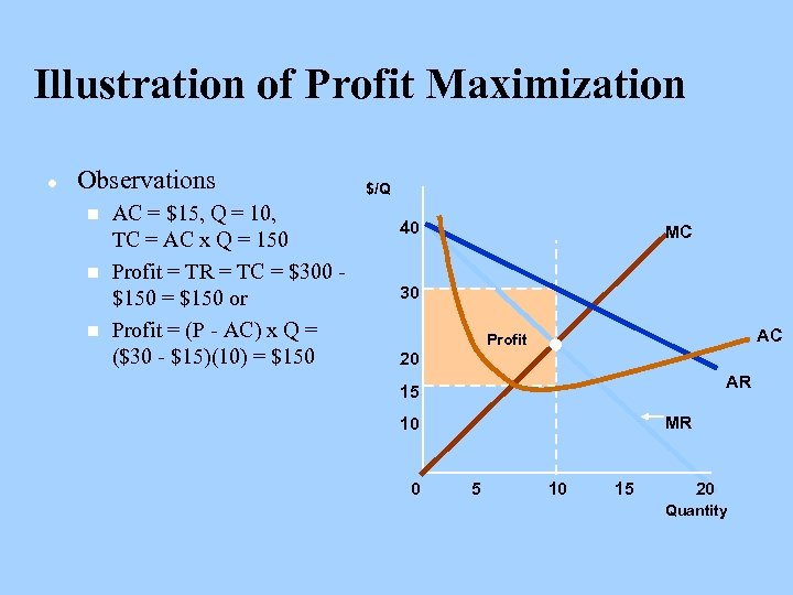Illustration of Profit Maximization l Observations n n n AC = $15, Q = 10, TC = AC x Q = 150 Profit = TR = TC = $300 $150 = $150 or Profit = (P - AC) x Q = ($30 - $15)(10) = $150 $/Q 40 MC 30 AC Profit 20 AR 15 MR 10 0 5 10 15 20 Quantity

Markup Rules l l l Two models of pricing – Markup over costs and What the market will bear. In fact they come together in a demandbased approach to markup pricing. How should price relate to cost to maximize profits?

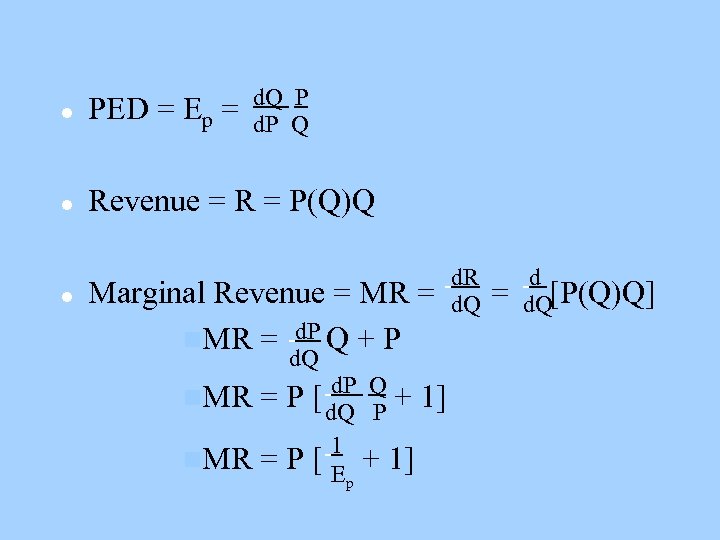d. Q P d. P Q l PED = Ep = l Revenue = R = P(Q)Q l Marginal Revenue = MR = n. MR = d. P Q + P d. Q n. MR d. P = P [ d. Q n. MR 1 Ep =P[ Q P + 1] d. R d. Q = d d. Q[P(Q)Q]

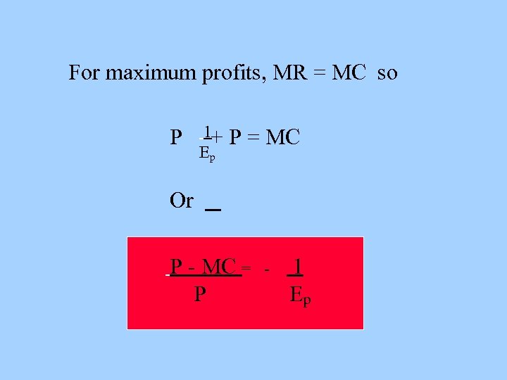For maximum profits, MR = MC so P 1+ Ep P = MC Or P - MC = P - 1 Ep

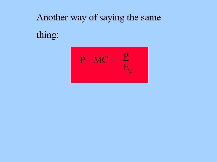Another way of saying the same thing: P - MC = - P Ep

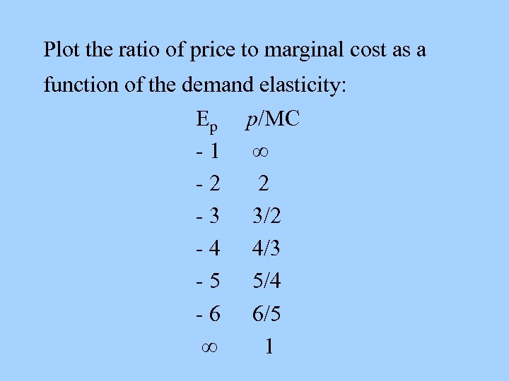Plot the ratio of price to marginal cost as a function of the demand elasticity: Ep -1 -2 -3 -4 -5 -6 p/MC 2 3/2 4/3 5/4 6/5 1

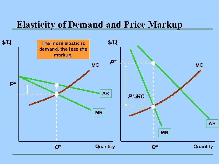Elasticity of Demand Price Markup $/Q The more elastic is demand, the less the markup. P* MC MC P* AR P*-MC MR AR MR Q* Quantity

Summary l This is a model of price setting as a markup over costs with the markup reflecting what the market will bear.

Switching costs ( “lock-in”) l l l These are the costs to consumers of switching from one producer or brand to another They make demand for the first brand less elastic less responsive to lower prices by competitors Switching costs associated with your competitors’ brands make your selling costs higher

Examples of switching costs: l l l Frequent flier bonuses and other rewards for loyalty Emphasis on “relationships” rather than “transactions”. Valid for banking, computer systems (custom jobs vs. off-the-shelf software), consulting, legal services Emphasis on “uniqueness” of product

Examples of Switching Costs l IBM with mainframes l ATT with PBXs l Microsoft with Windows

Switching Costs l l Can be high for widely-used software because of need to retrain, modify file formats, maintain links to other applications, etc. Hence incoming products will attempt to maintain compatibility and reduce these costs.

1. In general, a major role of marketing strategy and image building is to increase the costs of switching from your product, so as to make demand less elastic. 2. Switching costs are reflected in the PED. 3. Being an industry standard raises switching costs.

Consumer Surplus l With a downward sloping demand curve, and uniform price for all buyers, some buyers will be paying less than they are willing to pay for the good (for example, the buyers at the top left hand end of the demand curve)

l The difference between what a buyer is willing to pay for the units of a good which she buys, and the amount she actually pays, is called the buyer’s consumer surplus

One of the main aims of pricing strategy is to find a way of charging for goods which brings this consumer surplus to the seller. To quote the marketing SVP of American Airlines, “Why sell a seat for $200 to someone who is willing to pay $500 for it? ”

Consumer surplus & demand curve l l l Buyer’s consumer surplus is area beneath her demand curve and above horizontal line whose height is the price. Example - buyer is willing to pay $10 for 1 st unit, $9 for 2 nd, $8 for 3 rd, $7 for 4 th, etc. Construct demand curve.

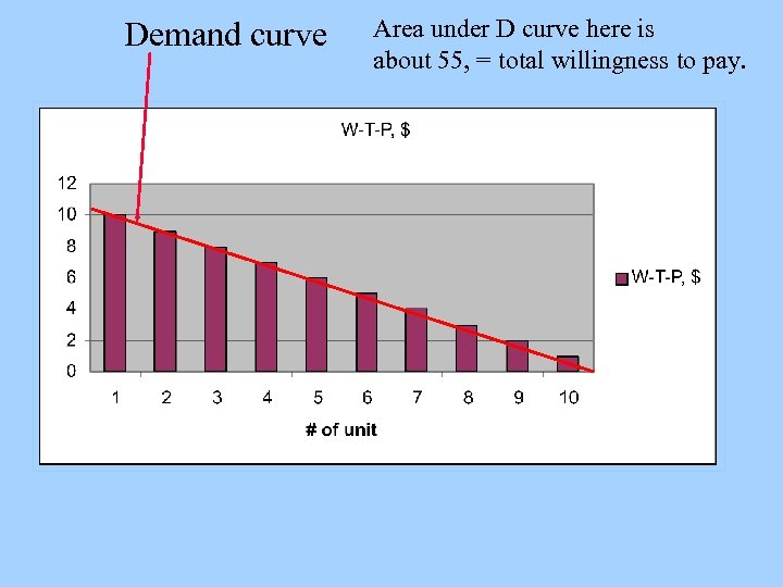Demand curve Area under D curve here is about 55, = total willingness to pay.

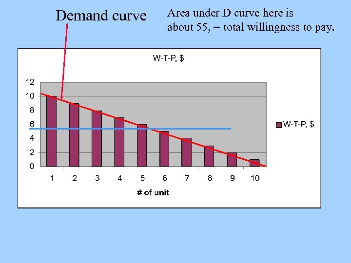
Consumer Surplus l l l Suppose price is zero. She will buy 10 units and consumer surplus is $(10+9+8+7+6 … ) which is $55. Area beneath demand curve and above P=0 is 1/2 x 10. 5 which is 55. 125. Try second example: price is just less than $6, so she buys 5 units. Pays $5 x 6 = $30.

Demand curve Area under D curve here is about 55, = total willingness to pay.

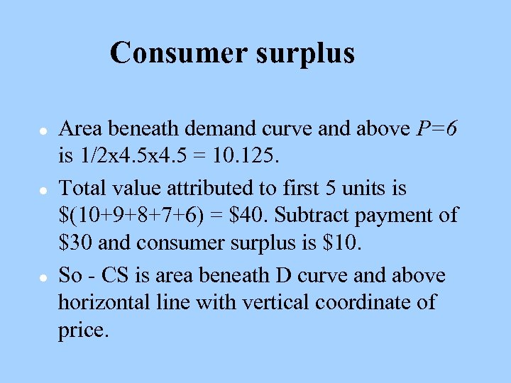Consumer surplus l l l Area beneath demand curve and above P=6 is 1/2 x 4. 5 = 10. 125. Total value attributed to first 5 units is $(10+9+8+7+6) = $40. Subtract payment of $30 and consumer surplus is $10. So - CS is area beneath D curve and above horizontal line with vertical coordinate of price.

Tools of pricing strategy Three main tools: Price discrimination, two-part pricing and bundling (1) Price discrimination: charging different prices for essentially the same good to different buyers. Charge each what they are willing to pay.

Different types of price discrimination l l l Charging a different price to every buyer. Examples: Reuters Info Services, car sales Segmenting the market. Airlines with business vs. vacation travel, railroads with time-of-day pricing, phone companies with time-of-day pricing, retail stores pricing by location. price discrimination over time: introduce a product at a high price and reduce the price over time. Sell at a high price to the aficionados - e. g. high fi systems, new and more powerful computers

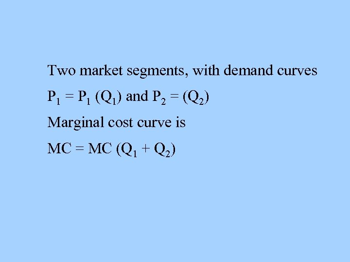Two market segments, with demand curves P 1 = P 1 (Q 1) and P 2 = (Q 2) Marginal cost curve is MC = MC (Q 1 + Q 2)

Market Segmentation l l Choose price, output so that MR same in each segment Common MR should equal MC

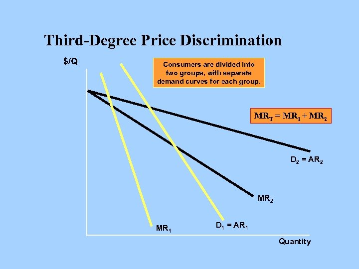Third-Degree Price Discrimination $/Q Consumers are divided into two groups, with separate demand curves for each group. MRT = MR 1 + MR 2 D 2 = AR 2 MR 1 D 1 = AR 1 Quantity

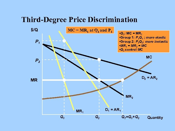Third-Degree Price Discrimination $/Q MC = MR 1 at Q 1 and P 1 • QT: MC = MRT • Group 1: P 1 Q 1 ; more elastic • Group 2: P 2 Q 2; more inelastic • MR 1 = MR 2 = MC • QT control MC MC P 2 D 2 = AR 2 MR MR 2 D 1 = AR 1 MR 1 Q 2 QT=Q 1+Q 2 Quantity

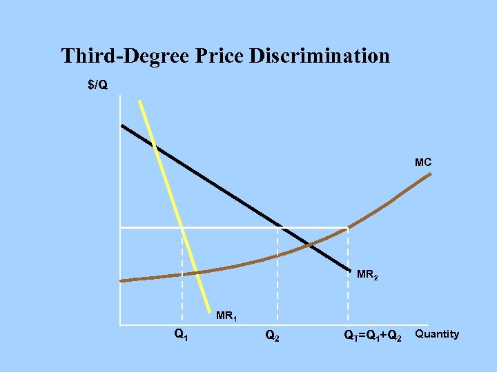Third-Degree Price Discrimination $/Q MC MR 2 MR 1 Q 2 QT=Q 1+Q 2 Quantity

Market Segmentation l l Choose price, output so that MR same in each segment Common MR should equal MC

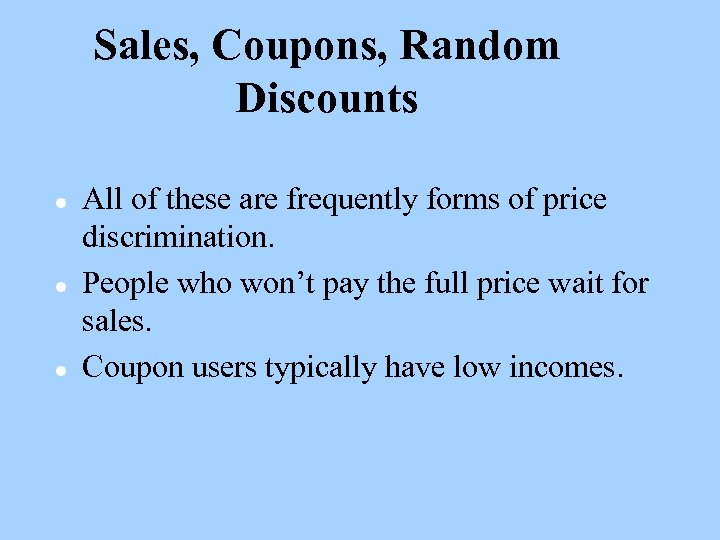Sales, Coupons, Random Discounts l l l All of these are frequently forms of price discrimination. People who won’t pay the full price wait for sales. Coupon users typically have low incomes.

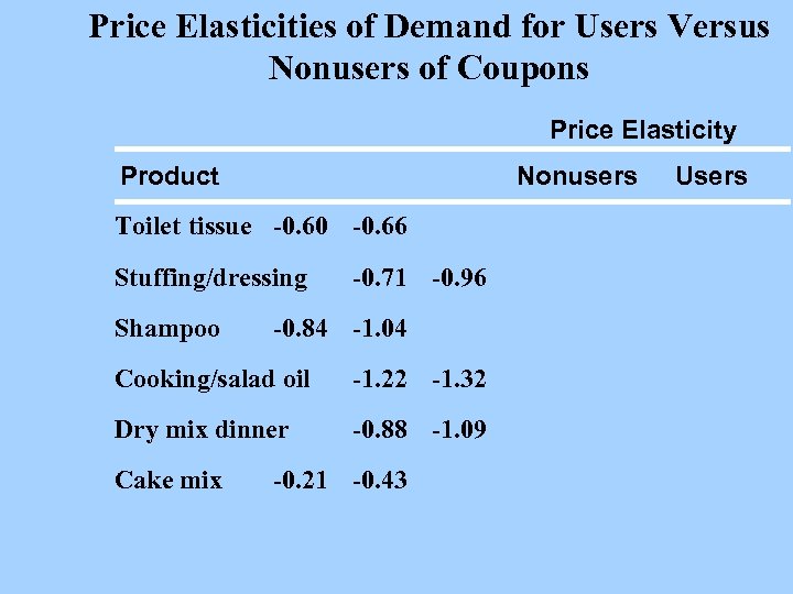Price Elasticities of Demand for Users Versus Nonusers of Coupons Price Elasticity Product Nonusers Toilet tissue -0. 60 -0. 66 Stuffing/dressing Shampoo -0. 71 -0. 96 -0. 84 -1. 04 Cooking/salad oil -1. 22 -1. 32 Dry mix dinner -0. 88 -1. 09 Cake mix -0. 21 -0. 43 Users

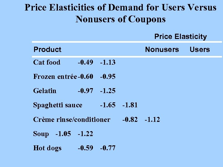Price Elasticities of Demand for Users Versus Nonusers of Coupons Price Elasticity Product Cat food Nonusers -0. 49 -1. 13 Frozen entrée-0. 60 -0. 95 Gelatin -0. 97 -1. 25 Spaghetti sauce -1. 65 -1. 81 Crème rinse/conditioner Soup -1. 05 -1. 22 Hot dogs -0. 59 -0. 77 -0. 82 -1. 12 Users

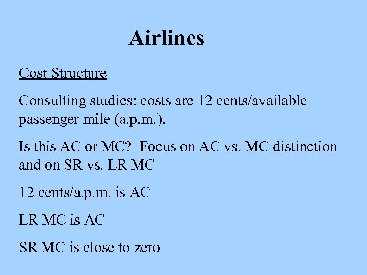Airlines Cost Structure Consulting studies: costs are 12 cents/available passenger mile (a. p. m. ). Is this AC or MC? Focus on AC vs. MC distinction and on SR vs. LR MC 12 cents/a. p. m. is AC LR MC is AC SR MC is close to zero

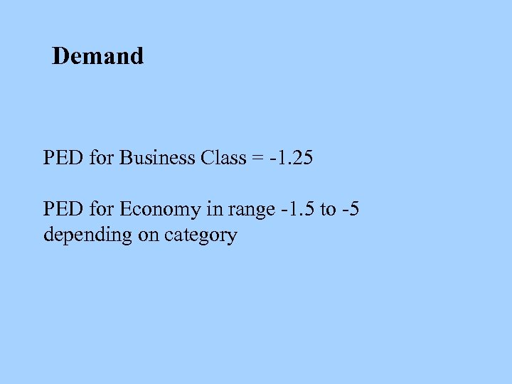Demand PED for Business Class = -1. 25 PED for Economy in range -1. 5 to -5 depending on category

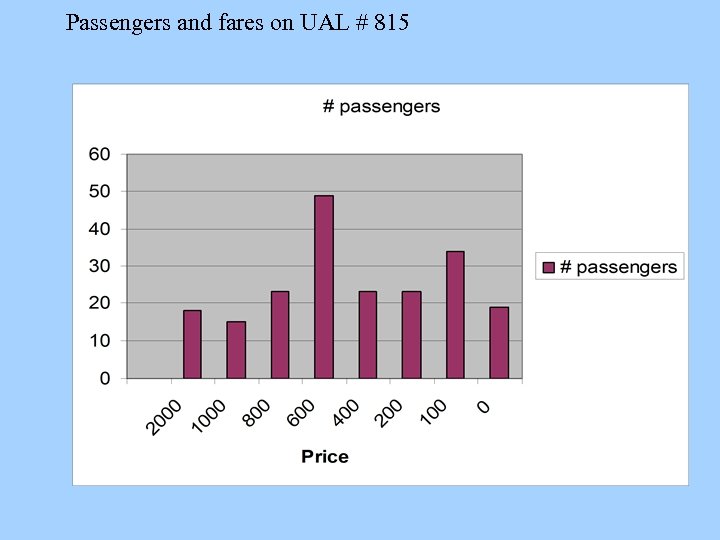Passengers and fares on UAL # 815

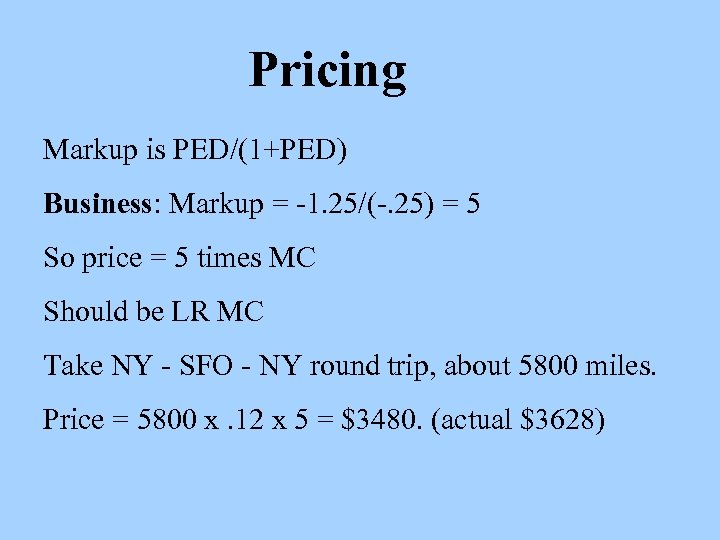Pricing Markup is PED/(1+PED) Business: Markup = -1. 25/(-. 25) = 5 So price = 5 times MC Should be LR MC Take NY - SFO - NY round trip, about 5800 miles. Price = 5800 x. 12 x 5 = $3480. (actual $3628)

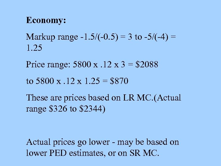Economy: Markup range -1. 5/(-0. 5) = 3 to -5/(-4) = 1. 25 Price range: 5800 x. 12 x 3 = $2088 to 5800 x. 12 x 1. 25 = $870 These are prices based on LR MC. (Actual range $326 to $2344) Actual prices go lower - may be based on lower PED estimates, or on SR MC.

What about situations where SR MC applies? Standby, bucket-shops, end-of-week specials. Examples of “Yield Management” - see also hotels, car rentals, etc. Also adjust prices for “load factor”. If this is 75%, actual revenues will be only 75% of that predicted by these prices so gross up price to allow for this.

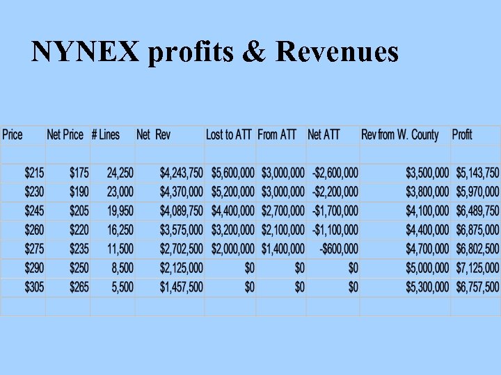
NYNEX Case

NYNEX profits & Revenues

The Two-Part Tariff l l The purchase of some products and services can be separated into two decisions, and therefore, two prices Decision to enter market and decision about how much to buy

The Two-Part Tariff l Examples 1) Amusement Park – Pay to enter – Pay for rides and food within the park 2) Tennis Club – Pay to join – Pay to play

The Two-Part Tariff l Examples 3) Rental of Mainframe Computers – Flat Fee – Processing Time 4) Safety Razor – Pay for razor – Pay for blades

The Two-Part Tariff l Examples 5) Polaroid Film – Pay for the camera – Pay for the film

The Two-Part Tariff l l Pricing decision is setting the entry fee (T) and the usage fee (P) Choosing the trade-off between free-entry and high user charges or high-entry and zero user charges

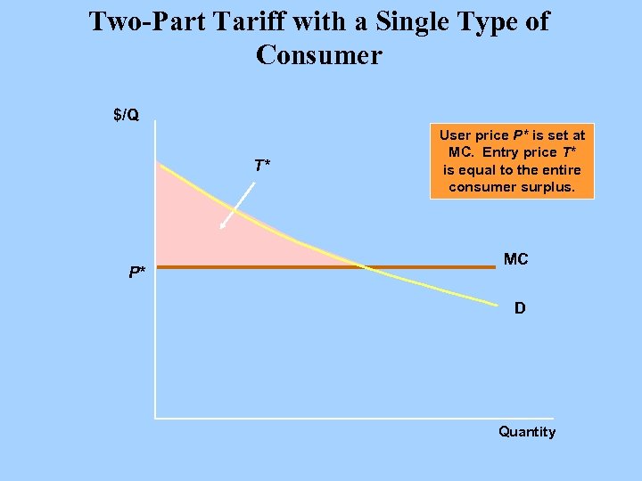Two-Part Tariff with a Single Type of Consumer $/Q T* P* User price P* is set at MC. Entry price T* is equal to the entire consumer surplus. MC D Quantity

Two-part tariffs with varied consumers: l l Consumer surplus of the lowest demand curve limits what you can charge as the fixed charge. If you charge more than this you lose this group of consumers. Try to devise ways of differentiating the fixed charges- see below about cell phones.

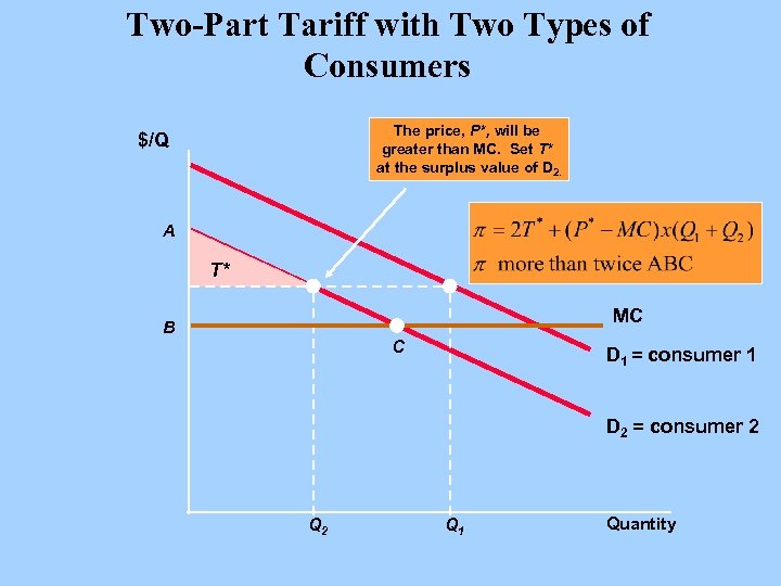Two-Part Tariff with Two Types of Consumers The price, P*, will be greater than MC. Set T* at the surplus value of D 2. $/Q A T* MC B C D 1 = consumer 1 D 2 = consumer 2 Q 1 Quantity

The Two-Part Tariff l The Two-Part Tariff With Many Different Consumers No exact way to determine P* and T*. n Must consider the trade-off between the entry fee T* and the use fee P*. n – Low entry fee: High sales and falling profit with lower price and more entrants.

The Two-Part Tariff l The Two-Part Tariff With Many Different Consumers To find optimum combination, choose several combinations of P, T. n Choose the combination that maximizes profit. n

The Two-Part Tariff l Rule of Thumb Similar demand: Choose P close to MC and high T n Dissimilar demand: Choose high P and low T. n

The Two-Part Tariff l Two-Part Tariff With A Twist n Entry price (T) entitles the buyer to a certain number of free units – Gillette razors with several blades – Amusement parks with some tokens – On-line with free time

Bundling l Selling several goods in one bundle n Hardware and software n Software suites n Auto accessories

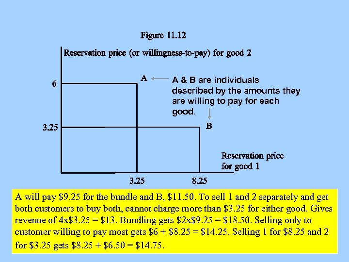A & B are individuals described by the amounts they are willing to pay for each good. A will pay $9. 25 for the bundle and B, $11. 50. To sell 1 and 2 separately and get both customers to buy both, cannot charge more than $3. 25 for either good. Gives revenue of 4 x$3. 25 = $13. Bundling gets $2 x$9. 25 = $18. 50. Selling only to customer willing to pay most gets $6 + $8. 25 = $14. 25. Selling 1 for $8. 25 and 2 for $3. 25 gets $8. 25 + $6. 50 = $14. 75.

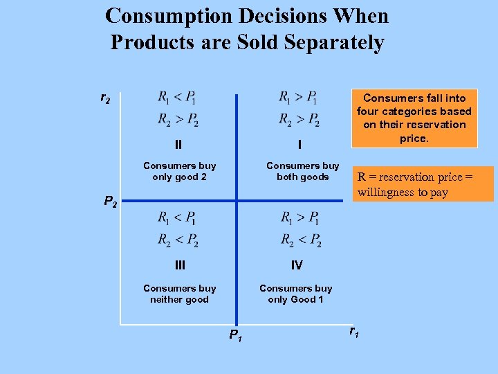Consumption Decisions When Products are Sold Separately r 2 II I Consumers buy only good 2 Consumers buy both goods P 2 III R = reservation price = willingness to pay IV Consumers buy neither good Consumers fall into four categories based on their reservation price. Consumers buy only Good 1 P 1 r 1

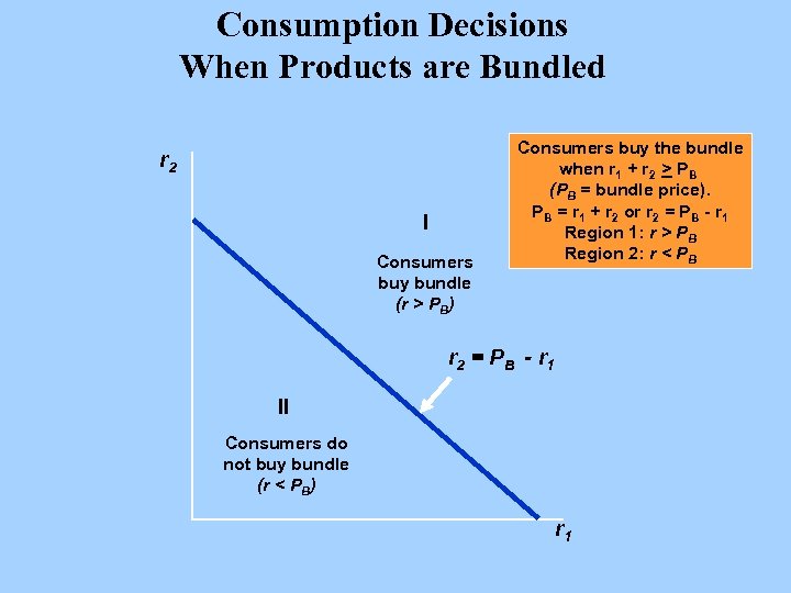Consumption Decisions When Products are Bundled r 2 I Consumers buy bundle (r > PB) Consumers buy the bundle when r 1 + r 2 > PB (PB = bundle price). PB = r 1 + r 2 or r 2 = PB - r 1 Region 1: r > PB Region 2: r < PB r 2 = P B - r 1 II Consumers do not buy bundle (r < PB) r 1

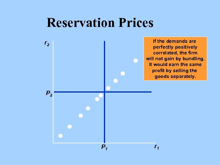Reservation Prices If the demands are perfectly positively correlated, the firm will not gain by bundling. It would earn the same profit by selling the goods separately. r 2 P 1 r 1

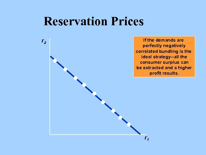Reservation Prices r 2 If the demands are perfectly negatively correlated bundling is the ideal strategy--all the consumer surplus can be extracted and a higher profit results. r 1

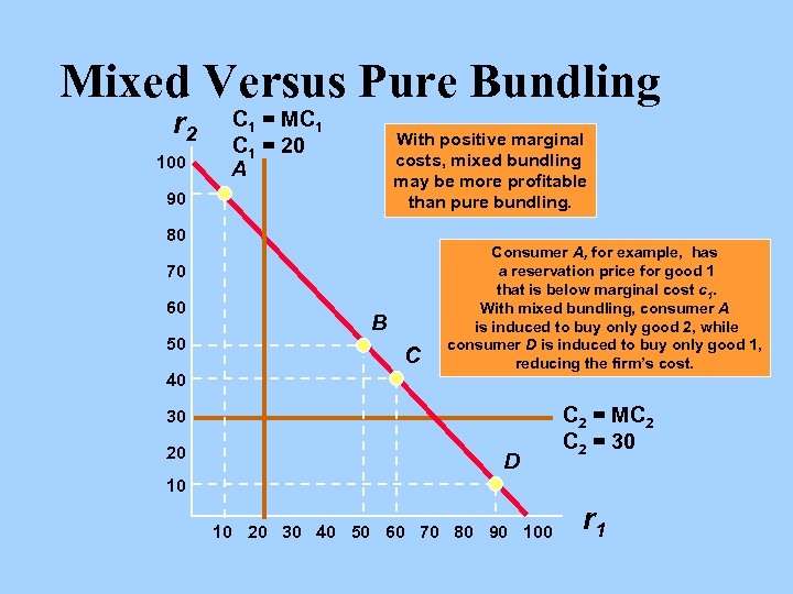Mixed Versus Pure Bundling r 2 100 C 1 = MC 1 = 20 A With positive marginal costs, mixed bundling may be more profitable than pure bundling. 90 80 70 60 50 40 B C Consumer A, for example, has a reservation price for good 1 that is below marginal cost c 1. With mixed bundling, consumer A is induced to buy only good 2, while consumer D is induced to buy only good 1, reducing the firm’s cost. 30 20 D C 2 = MC 2 = 30 10 10 20 30 40 50 60 70 80 90 100 r 1

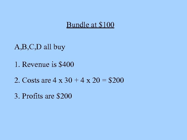Bundle at $100 A, B, C, D all buy 1. Revenue is $400 2. Costs are 4 x 30 + 4 x 20 = $200 3. Profits are $200

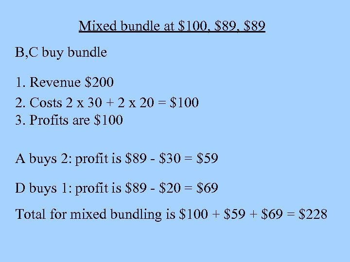Mixed bundle at $100, $89 B, C buy bundle 1. Revenue $200 2. Costs 2 x 30 + 2 x 20 = $100 3. Profits are $100 A buys 2: profit is $89 - $30 = $59 D buys 1: profit is $89 - $20 = $69 Total for mixed bundling is $100 + $59 + $69 = $228

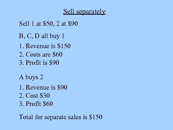Sell separately Sell 1 at $50, 2 at $90 B, C, D all buy 1 1. Revenue is $150 2. Costs are $60 3. Profit is $90 A buys 2 1. Revenue is $90 2. Cost $30 3. Profit $60 Total for separate sales is $150

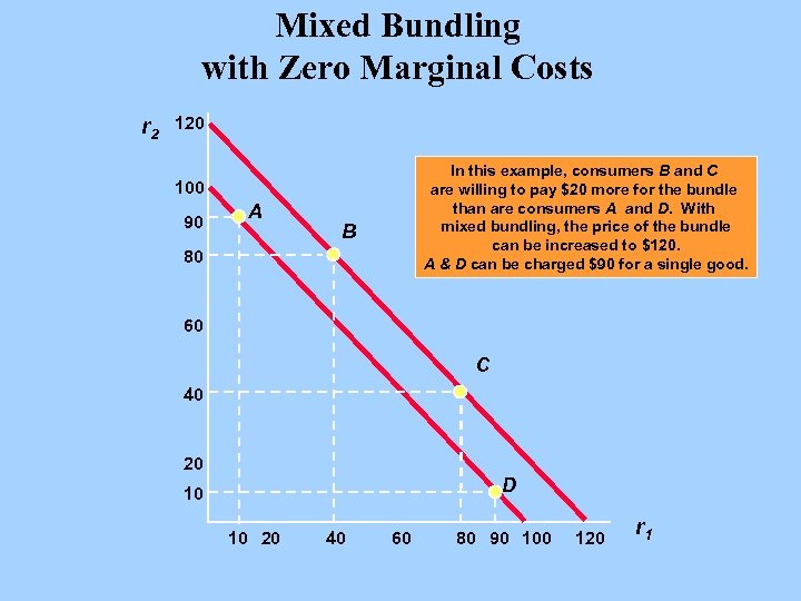Mixed Bundling with Zero Marginal Costs r 2 120 In this example, consumers B and C are willing to pay $20 more for the bundle than are consumers A and D. With mixed bundling, the price of the bundle can be increased to $120. A & D can be charged $90 for a single good. 100 90 A B 80 60 C 40 20 D 10 10 20 40 60 80 90 100 120 r 1

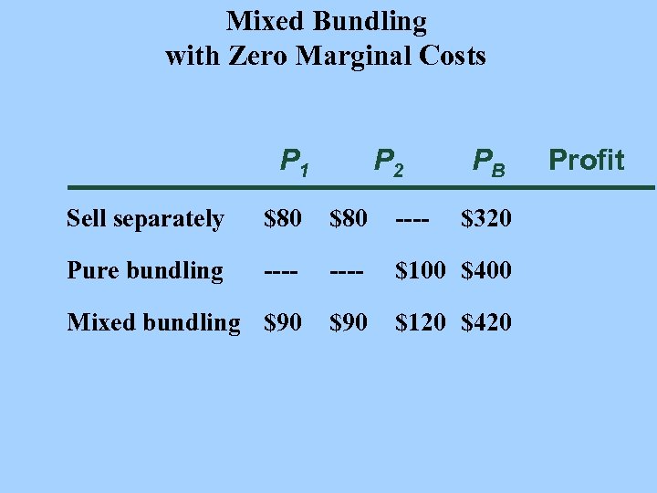Mixed Bundling with Zero Marginal Costs P 1 P 2 PB Sell separately $80 ---- $320 Pure bundling ---- $100 $400 Mixed bundling $90 $120 $420 Profit

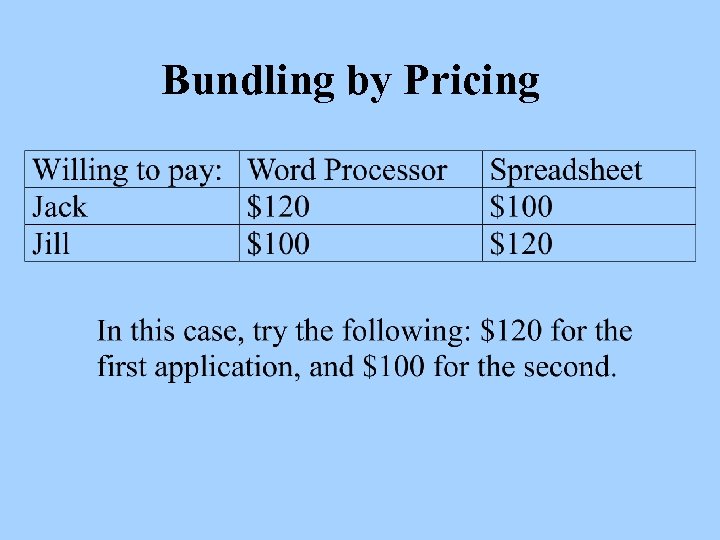Bundling by Pricing

Pricing Cell-Phones l l l A mix of discrimination, bundling and twopart pricing Buy the phone (connection/membership charge) & pay for service - like Polaroid, Gilette. Phones at different price points. Then you have a choice between several two -part tariffs

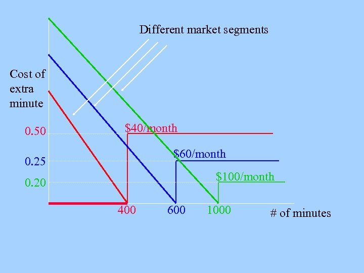
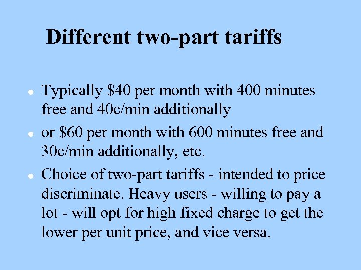Different two-part tariffs l l l Typically $40 per month with 400 minutes free and 40 c/min additionally or $60 per month with 600 minutes free and 30 c/min additionally, etc. Choice of two-part tariffs - intended to price discriminate. Heavy users - willing to pay a lot - will opt for high fixed charge to get the lower per unit price, and vice versa.

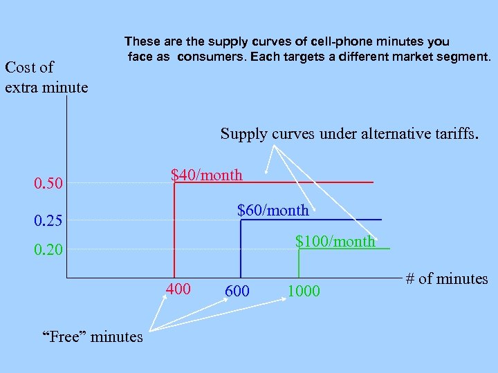Cost of extra minute These are the supply curves of cell-phone minutes you face as consumers. Each targets a different market segment. Supply curves under alternative tariffs. 0. 50 $40/month $60/month 0. 25 $100/month 0. 20 400 “Free” minutes 600 1000 # of minutes

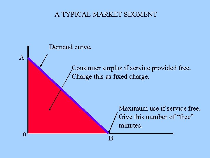
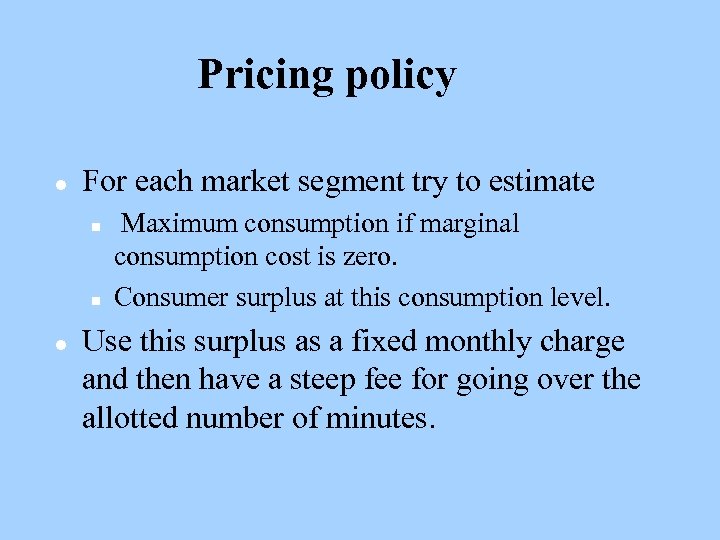Pricing policy l For each market segment try to estimate n n l Maximum consumption if marginal consumption cost is zero. Consumer surplus at this consumption level. Use this surplus as a fixed monthly charge and then have a steep fee for going over the allotted number of minutes.

A TYPICAL MARKET SEGMENT Demand curve. A Consumer surplus if service provided free. Charge this as fixed charge. Maximum use if service free. Give this number of “free” minutes. 0 B

Different market segments Cost of extra minute 0. 50 $40/month $60/month 0. 25 $100/month 0. 20 400 600 1000 # of minutes

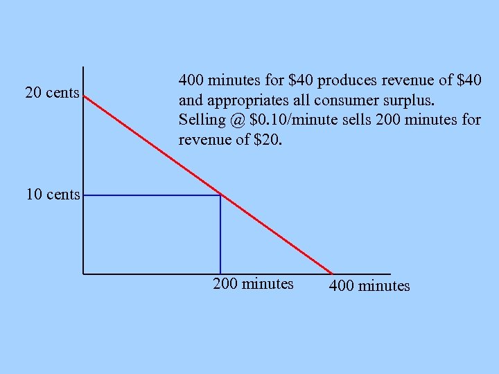
Key aspects of pricing policy l Compare n n l giving 400 minutes for $40 ($0. 10 per minute on average) with charging $0. 10 per minute for any number of minutes. If demand curve is as Verizon policy implies, then selling at $0. 10/minute will sell 100 minutes (next slide) and give revenue of $20, rather than $40

20 cents 400 minutes for $40 produces revenue of $40 and appropriates all consumer surplus. Selling @ $0. 10/minute sells 200 minutes for revenue of $20. 10 cents 200 minutes 400 minutes

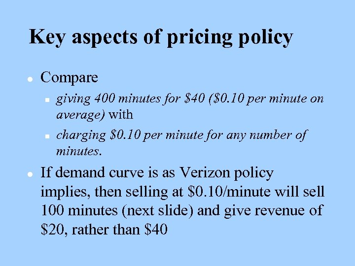
Key aspects l l l So selling 400 minutes for $40 is NOT the same as selling each minute at the average price, 40/400 = $0. 10. Selling the 400 minutes together is twice as profitable as selling each minute at $0. 10. WHY? Bundling earlier and later minutes together.

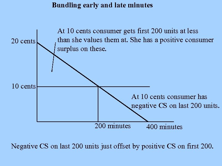Bundling early and late minutes 20 cents At 10 cents consumer gets first 200 units at less than she values them at. She has a positive consumer surplus on these. 10 cents At 10 cents consumer has negative CS on last 200 units. 200 minutes 400 minutes Negative CS on last 200 units just offset by positive CS on first 200.

Conclusions l l l Key aspect of pricing here is bundling early and late minutes. Positive CS on former offsets negative CS on latter. Prices seem to be low - probably competition between different carriers and between cell phones and normal phones. Carriers see market share as critical in growing market. Valued “per pop. ”

Pricing of AIDS Drugs l l l Key issue – price discrimination by country is natural as country is a proxy for income and WTP. Deal struck with SA and other poor countries is no more than extension of this principle. Leads to situation where rich countries naturally contribute more to R&D expenses and so in effect subsidize others.

Pricing AIDS Drugs l May make economic sense to sell to poorest markets at less than average cost as long as price above marginal cost

Limiting Market Power: The U. S. Antitrust Laws l Antitrust Laws: Promote a competitive economy - competition benefits consumers. n Rules and regulations designed to promote a competitive economy by: n – Prohibiting actions that restrain or are likely to restrain competition – Restricting the forms of market structures that are allowable (e. g. excessive concentration).

Limiting Market Power: The U. S. Antitrust Laws l Sherman Act (1890) n Section 1 – Prohibits contracts, combinations, or conspiracies in restraint of trade l Explicit agreement to restrict output or fix prices l Implicit collusion through parallel conduct

Limiting Market Power: The U. S. Antitrust Laws Examples of Illegal Combinations l 1983 n l Six companies and six executives indicted for price of copper tubing 1996 n Archer Daniels Midland (ADM) pleaded guilty to price fixing for lysine -- three sentenced to prison in 1999

Limiting Market Power: The U. S. Antitrust Laws Examples of Illegal Combinations l 1999 n Roche A. G. , BASF A. G. , Rhone-Poulenc and Takeda pleaded guilty to price fixing of vitamins -- fined more than $1 billion.

Limiting Market Power: The U. S. Antitrust Laws l Sherman Act (1890) n Section 2 – Makes it illegal to monopolize or attempt to monopolize a market and prohibits conspiracies that result in monopolization.

Limiting Market Power: The U. S. Antitrust Laws l Clayton Act (1914) 1) Makes it unlawful to require a buyer or lessor not to buy from a competitor 2) Prohibits predatory pricing

Limiting Market Power: The U. S. Antitrust Laws l l Clayton Act (1914) Prohibits mergers and acquisitions if they “substantially lessen competition”or “tend to create a monopoly” Proposed mergers have to be approved by the Justice Department.

Limiting Market Power: The U. S. Antitrust Laws l Robinson-Patman Act (1936) Prohibits price discrimination if it is likely to injure the competition n Also new case on Acuvue Contact Lenses 2002 n

Limiting Market Power: The U. S. Antitrust Laws l Federal Trade Commission Act (1914, amended 1938, 1973, 1975) 1) Created the Federal Trade Commission (FTC) 2) Prohibitions against deceptive advertising, labeling, agreements with retailer to exclude competing brands

Limiting Market Power: The U. S. Antitrust Laws l Antitrust laws are enforced three ways: 1) Antitrust Division of the Department of Justice – A part of the executive branch--the administration can influence enforcement – Fines levied on businesses; fines and imprisonment levied on individuals

Limiting Market Power: The U. S. Antitrust Laws l Antitrust laws are enforced three ways: 2) Federal Trade Commission – Enforces through voluntary understanding or formal commission order

Limiting Market Power: The U. S. Antitrust Laws l Antitrust laws are enforced three ways: 3) Private Proceedings – Lawsuits for damages – Plaintiff can receive treble damages

Limiting Market Power: The U. S. Antitrust Laws l Two Examples n n American Airlines -- Price fixing Microsoft – Monopoly power – Predatory actions – Collusion

Recent cases l l GE and Honeywell United Airlines and US Airways Mergers blocked on grounds of restriction of competition. Bundling an issue for Microsoft – but because of its anti-competitive implications,