Pricing Strategies Some pricing strategies that we

Pricing Strategies

Some pricing strategies that we will explore: 1. 2. 3. 4. 5. 6. 7. 8. Price discrimination – 1 st, 2 nd, & 3 rd degree “Two-part Tariff” pricing Bundling Advertising Cost-plus markup pricing Product Lines Peak-Load pricing Transfer Pricing

Price Discrimination • Charging different prices to different consumers for the same product. • Enables firms to charge some consumers higher prices, and to capture consumer surplus.

Under what conditions is price discrimination possible? a. Firm must have some control over price. b. The firm can identify different submarkets. c. The submarkets have different price elasticities of demand. d. The firm can prevent arbitrage (the purchase of an item for immediate resale in order to profit from the price discrepancy).

3 Types of Price Discrimination First Degree Each customer is charged the maximum price that they are willing to pay. Second Degree – involves self-selection One type of 2 nd degree price discrimination is block pricing or quantity discounts in which firms charge different prices depending on volume of usage. Third Degree or multi-market (most common) Markets distinguished by other factors.

Since under first degree price discrimination, each customer is charged the maximum price that they are willing to pay, consumer surplus is zero.

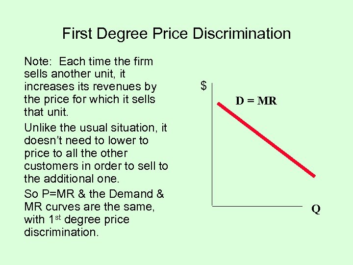First Degree Price Discrimination Note: Each time the firm sells another unit, it increases its revenues by the price for which it sells that unit. Unlike the usual situation, it doesn’t need to lower to price to all the other customers in order to sell to the additional one. So P=MR & the Demand & MR curves are the same, with 1 st degree price discrimination. $ D = MR Q

First degree price discrimination Example: Suppose the demand curve for a monopolist’s product is: P = 9 – 0. 005 Q. The average total cost curve is a horizontal line: ATC = MC = 1. 5 (1) Determine the price, quantity, consumer surplus, producer surplus (profit), & the sum of consumer & producer surplus, if the firm does NOT price discriminate. (2) Determine the quantity, consumer surplus, producer surplus (profit), & the sum of consumer & producer surplus, if the firm does price discriminate.

First, if the firm does NOT price discriminate: We have the demand curve for a monopolist’s product is: P = 9 – 0. 005 Q. & the average total cost curve is: ATC = MC = 1. 5 TR = PQ =(9 – 0. 005 Q) Q = 9 Q – 0. 005 Q 2. Then MR = d. TR/d. Q = 9 – 0. 01 Q. Setting MR = MC, we have 9 – 0. 01 Q = 1. 5 or 7. 5 = 0. 01 Q. So Q = 750, & P = 9 – 0. 005 Q = 9 – 0. 005 (750) = 5. 25. Profit or producer surplus = TR – TC = PQ – (ATC)Q = (5. 25)(750) – (1. 5)(750) = 2812. 5

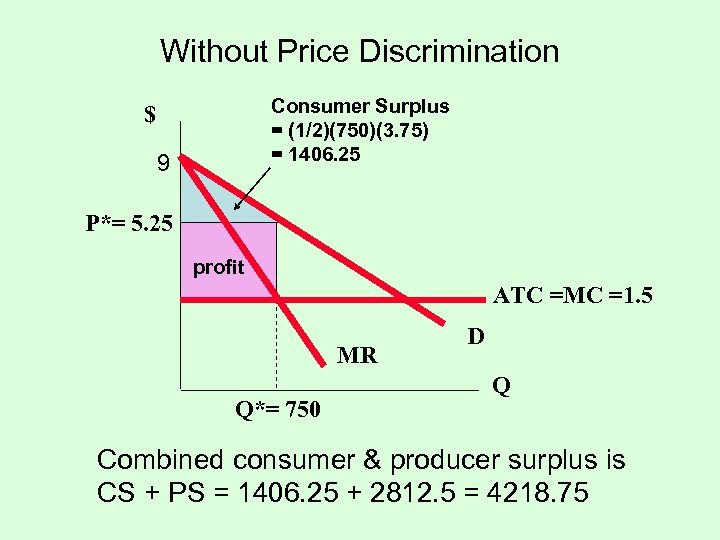Without Price Discrimination Consumer Surplus = (1/2)(750)(3. 75) = 1406. 25 $ 9 P*= 5. 25 profit ATC =MC =1. 5 MR Q*= 750 D Q Combined consumer & producer surplus is CS + PS = 1406. 25 + 2812. 5 = 4218. 75

Now if the firm does 1 st degree price discrimination: We had the demand curve: P = 9 – 0. 005 Q, & the average total cost curve: ATC = MC = 1. 5 MR is now the same as the demand function, so MR = 9 – 0. 005 Q. Setting MR = MC, we have 9 – 0. 005 Q = 1. 5 or 7. 5 = 0. 005 Q. So Q = 1500.

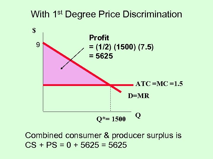With 1 st Degree Price Discrimination $ 9 Profit = (1/2) (1500) (7. 5) = 5625 ATC =MC =1. 5 D=MR Q*= 1500 Q Combined consumer & producer surplus is CS + PS = 0 + 5625 = 5625

2 nd Degree Price Discrimination: Block Pricing Price is based on volume of usage of the good. Those who consume large quantities are charged a lower price. Those consuming small quantities are charged a higher price.

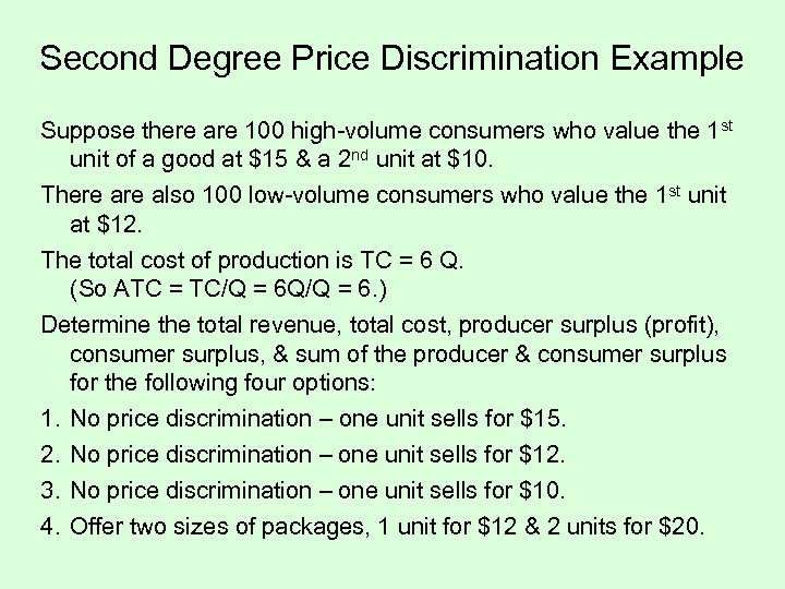Second Degree Price Discrimination Example Suppose there are 100 high-volume consumers who value the 1 st unit of a good at $15 & a 2 nd unit at $10. There also 100 low-volume consumers who value the 1 st unit at $12. The total cost of production is TC = 6 Q. (So ATC = TC/Q = 6 Q/Q = 6. ) Determine the total revenue, total cost, producer surplus (profit), consumer surplus, & sum of the producer & consumer surplus for the following four options: 1. 2. 3. 4. No price discrimination – one unit sells for $15. No price discrimination – one unit sells for $12. No price discrimination – one unit sells for $10. Offer two sizes of packages, 1 unit for $12 & 2 units for $20.

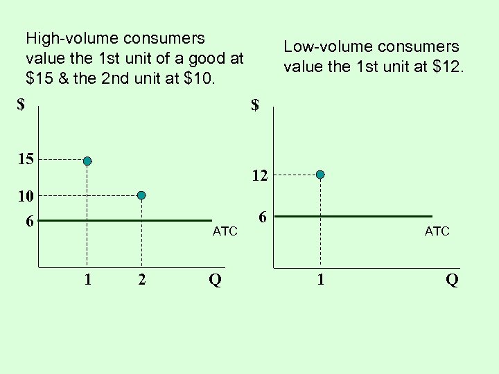High-volume consumers value the 1 st unit of a good at $15 & the 2 nd unit at $10. $ Low-volume consumers value the 1 st unit at $12. $ 15 12 10 6 ATC 1 2 Q 6 ATC 1 Q

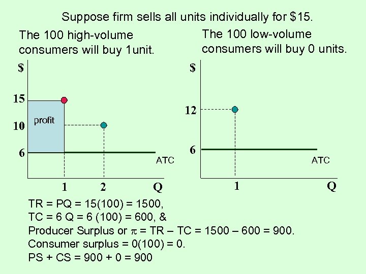Suppose firm sells all units individually for $15. The 100 low-volume The 100 high-volume consumers will buy 0 units. consumers will buy 1 unit. $ $ 15 10 12 profit 6 ATC 1 2 Q 6 ATC 1 TR = PQ = 15(100) = 1500, TC = 6 Q = 6 (100) = 600, & Producer Surplus or = TR – TC = 1500 – 600 = 900. Consumer surplus = 0(100) = 0. PS + CS = 900 + 0 = 900 Q

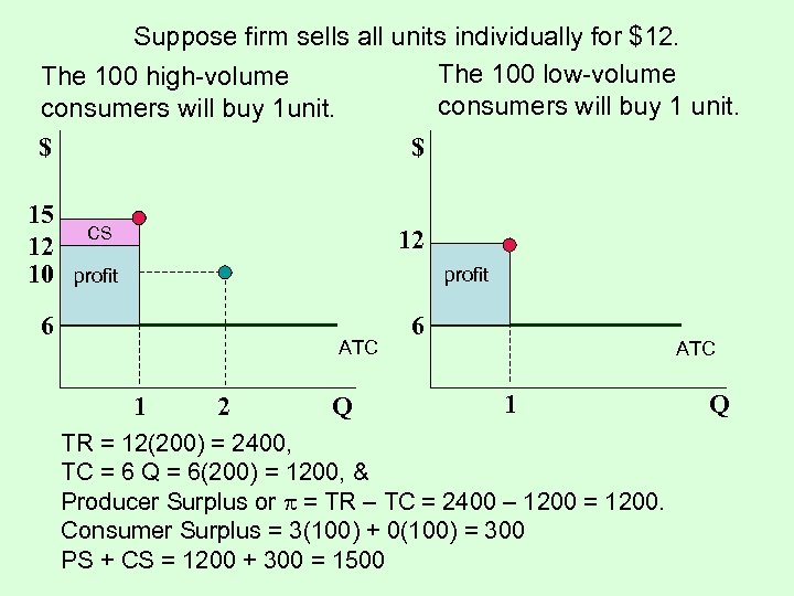Suppose firm sells all units individually for $12. The 100 low-volume The 100 high-volume consumers will buy 1 unit. consumers will buy 1 unit. $ $ 15 12 10 CS 12 profit 6 ATC 1 2 Q 6 ATC 1 TR = 12(200) = 2400, TC = 6 Q = 6(200) = 1200, & Producer Surplus or = TR – TC = 2400 – 1200 = 1200. Consumer Surplus = 3(100) + 0(100) = 300 PS + CS = 1200 + 300 = 1500 Q

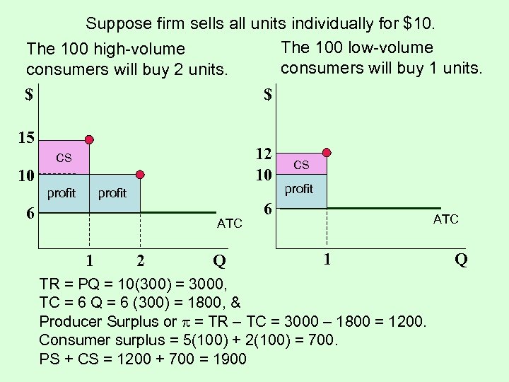Suppose firm sells all units individually for $10. The 100 low-volume The 100 high-volume consumers will buy 1 units. consumers will buy 2 units. $ $ 15 12 10 CS 10 profit 6 ATC 1 2 Q CS profit 6 ATC 1 TR = PQ = 10(300) = 3000, TC = 6 Q = 6 (300) = 1800, & Producer Surplus or = TR – TC = 3000 – 1800 = 1200. Consumer surplus = 5(100) + 2(100) = 700. PS + CS = 1200 + 700 = 1900 Q

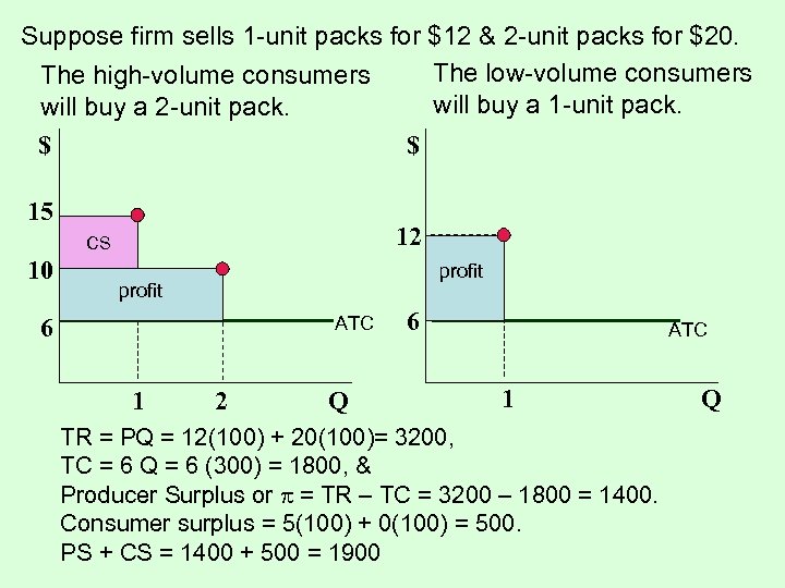Suppose firm sells 1 -unit packs for $12 & 2 -unit packs for $20. The low-volume consumers The high-volume consumers will buy a 1 -unit pack. will buy a 2 -unit pack. $ $ 15 12 CS 10 profit ATC 6 1 2 Q 6 ATC 1 TR = PQ = 12(100) + 20(100)= 3200, TC = 6 Q = 6 (300) = 1800, & Producer Surplus or = TR – TC = 3200 – 1800 = 1400. Consumer surplus = 5(100) + 0(100) = 500. PS + CS = 1400 + 500 = 1900 Q

In our 2 nd degree price discrimination case, the firm offered two sizes of packages, 1 unit for $12 & 2 units for $20. The 100 high-volume consumers value the 1 st unit of a good at $15 & the 2 nd unit at $10. However, notice that if the firm tried to charge $25 for the 2 -pack, the high-volume consumers would only buy a 1 -pack. This is because they would be better off with consumer surplus of $15 – $12 = 3 with a 1 -pack than consumer surplus of $25 – $25 = 0 with a 2 -pack. The profit with 2 nd order price discrimination is more than the profit for the one-price options. PS+CS is the same as for the unit price of $10, but the producer has captured the $200 lowvolume CS as PS or profit.

Third Degree Price Discrimination Charging different prices to different groups. Example: Charging lower movie admissions to students & senior citizens than to other moviegoers.

Third Degree Price Discrimination For each group, the firm produces such that MR = MC. The group with the lowest elasticity pays the highest price. Example: Students & senior citizens may have more limited incomes, and therefore be more responsive to changes in movie prices. Other movie-goers may be less responsive to changes in movie prices.

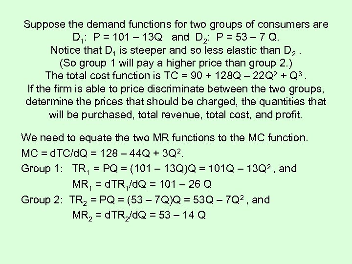Suppose the demand functions for two groups of consumers are D 1: P = 101 – 13 Q and D 2: P = 53 – 7 Q. Notice that D 1 is steeper and so less elastic than D 2. (So group 1 will pay a higher price than group 2. ) The total cost function is TC = 90 + 128 Q – 22 Q 2 + Q 3. If the firm is able to price discriminate between the two groups, determine the prices that should be charged, the quantities that will be purchased, total revenue, total cost, and profit. We need to equate the two MR functions to the MC function. MC = d. TC/d. Q = 128 – 44 Q + 3 Q 2. Group 1: TR 1 = PQ = (101 – 13 Q)Q = 101 Q – 13 Q 2 , and MR 1 = d. TR 1/d. Q = 101 – 26 Q Group 2: TR 2 = PQ = (53 – 7 Q)Q = 53 Q – 7 Q 2 , and MR 2 = d. TR 2/d. Q = 53 – 14 Q

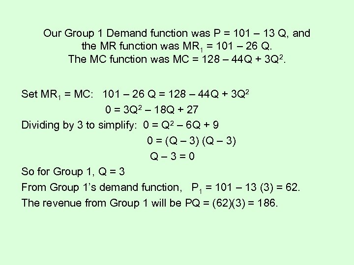Our Group 1 Demand function was P = 101 – 13 Q, and the MR function was MR 1 = 101 – 26 Q. The MC function was MC = 128 – 44 Q + 3 Q 2. Set MR 1 = MC: 101 – 26 Q = 128 – 44 Q + 3 Q 2 0 = 3 Q 2 – 18 Q + 27 Dividing by 3 to simplify: 0 = Q 2 – 6 Q + 9 0 = (Q – 3) Q– 3=0 So for Group 1, Q = 3 From Group 1’s demand function, P 1 = 101 – 13 (3) = 62. The revenue from Group 1 will be PQ = (62)(3) = 186.

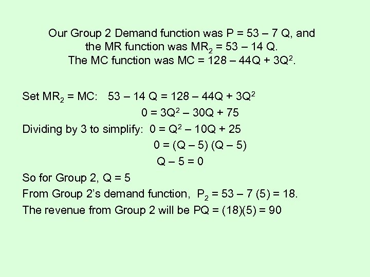Our Group 2 Demand function was P = 53 – 7 Q, and the MR function was MR 2 = 53 – 14 Q. The MC function was MC = 128 – 44 Q + 3 Q 2. Set MR 2 = MC: 53 – 14 Q = 128 – 44 Q + 3 Q 2 0 = 3 Q 2 – 30 Q + 75 Dividing by 3 to simplify: 0 = Q 2 – 10 Q + 25 0 = (Q – 5) Q– 5=0 So for Group 2, Q = 5 From Group 2’s demand function, P 2 = 53 – 7 (5) = 18. The revenue from Group 2 will be PQ = (18)(5) = 90

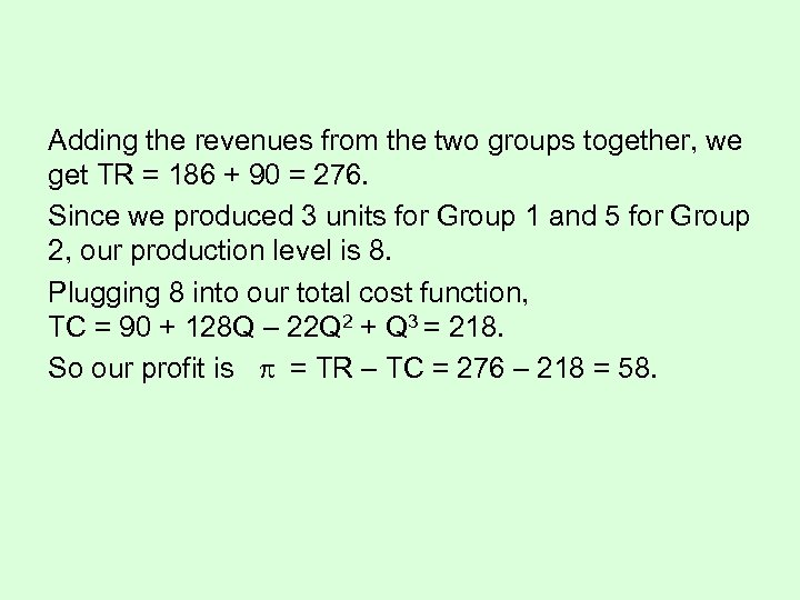Adding the revenues from the two groups together, we get TR = 186 + 90 = 276. Since we produced 3 units for Group 1 and 5 for Group 2, our production level is 8. Plugging 8 into our total cost function, TC = 90 + 128 Q – 22 Q 2 + Q 3 = 218. So our profit is = TR – TC = 276 – 218 = 58.

The “Two-Part Tariff” There are two components to the price: a unit price (P) for each unit consumed, & a “tariff” (T) for entry into the market. Examples include BJ’s, telephone service, health clubs, etc. The tariff enables the firm to capture some consumer surplus.

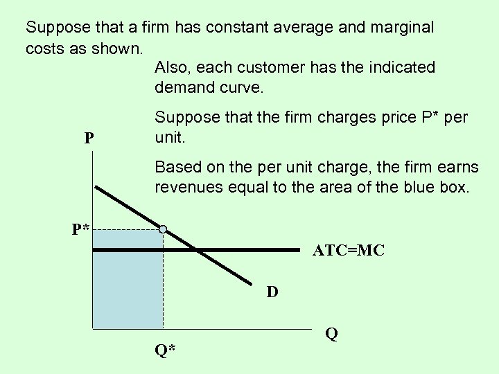Suppose that a firm has constant average and marginal costs as shown. Also, each customer has the indicated demand curve. P Suppose that the firm charges price P* per unit. Based on the per unit charge, the firm earns revenues equal to the area of the blue box. P* ATC=MC D Q* Q

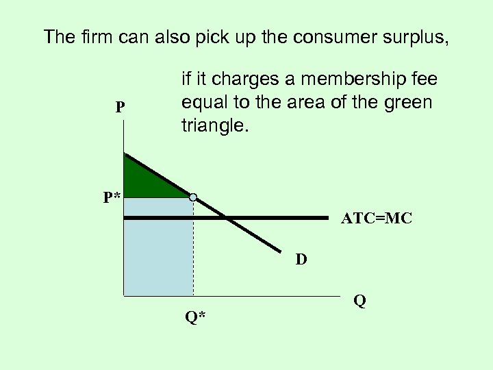The firm can also pick up the consumer surplus, P if it charges a membership fee equal to the area of the green triangle. P* ATC=MC D Q* Q

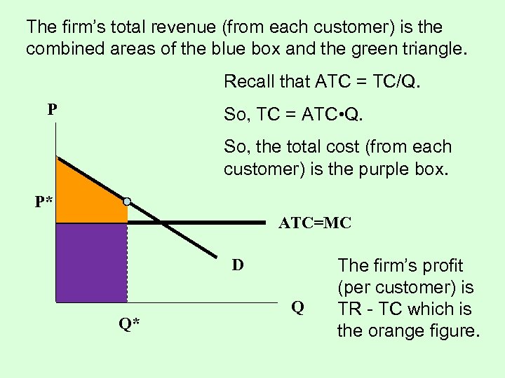The firm’s total revenue (from each customer) is the combined areas of the blue box and the green triangle. Recall that ATC = TC/Q. P So, TC = ATC • Q. So, the total cost (from each customer) is the purple box. P* ATC=MC D Q* Q The firm’s profit (per customer) is TR - TC which is the orange figure.

The firm’s profit from this two-part tariff strategy will be greatest if it produces where the Demand ATC = MC curves intersect, or P = ATC = MC. P P* ATC=MC D Q* Q

Two-Part Tariff Example Suppose a firm’s TC function is TC = 5 Q. Suppose also that each of the firm’s customers has this demand curve: P = 35 – Q. Determine the appropriate unit price and membership fee for a two-part tariff pricing strategy. Also determine the quantity purchased, total revenue, total cost, and profit per customer.

Demand function (for each person): P = 35 – Q Total cost function: TC = 5 Q As we indicated previously, the firm’s profit will be greatest if it produces where P = ATC = MC = 5 So, P = 35 – Q = 5 , So, 30 = Q. So revenue person from per unit sales is PQ = (5)(30) = 150. Next we need to determine the appropriate membership fee.

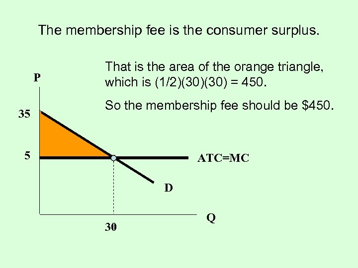The membership fee is the consumer surplus. P 35 That is the area of the orange triangle, which is (1/2)(30) = 450. So the membership fee should be $450. 5 ATC=MC D 30 Q

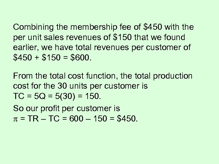Combining the membership fee of $450 with the per unit sales revenues of $150 that we found earlier, we have total revenues per customer of $450 + $150 = $600. From the total cost function, the total production cost for the 30 units per customer is TC = 5 Q = 5(30) = 150. So our profit per customer is = TR – TC = 600 – 150 = $450.

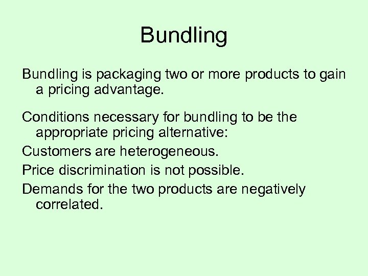Bundling is packaging two or more products to gain a pricing advantage. Conditions necessary for bundling to be the appropriate pricing alternative: Customers are heterogeneous. Price discrimination is not possible. Demands for the two products are negatively correlated.

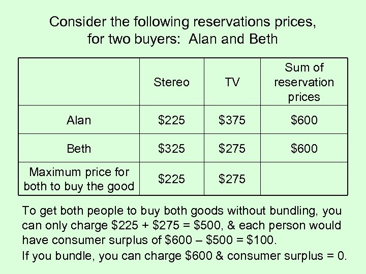Consider the following reservations prices, for two buyers: Alan and Beth Stereo TV Sum of reservation prices Alan $225 $375 $600 Beth $325 $275 $600 Maximum price for both to buy the good $225 $275 To get both people to buy both goods without bundling, you can only charge $225 + $275 = $500, & each person would have consumer surplus of $600 – $500 = $100. If you bundle, you can charge $600 & consumer surplus = 0.

The effectiveness of bundling as a pricing strategy depends upon the degree of negative correlation between the demands for the two goods.

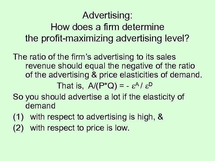Advertising: How does a firm determine the profit-maximizing advertising level? The ratio of the firm’s advertising to its sales revenue should equal the negative of the ratio of the advertising & price elasticities of demand. That is, A/(P*Q) = - A / D So you should advertise a lot if the elasticity of demand (1) with respect to advertising is high, & (2) with respect to price is low.

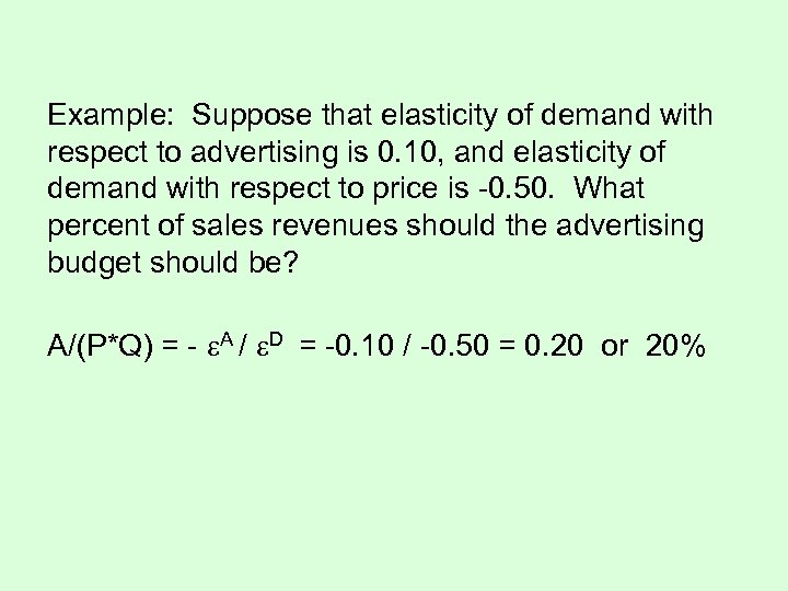Example: Suppose that elasticity of demand with respect to advertising is 0. 10, and elasticity of demand with respect to price is -0. 50. What percent of sales revenues should the advertising budget should be? A/(P*Q) = - A / D = -0. 10 / -0. 50 = 0. 20 or 20%

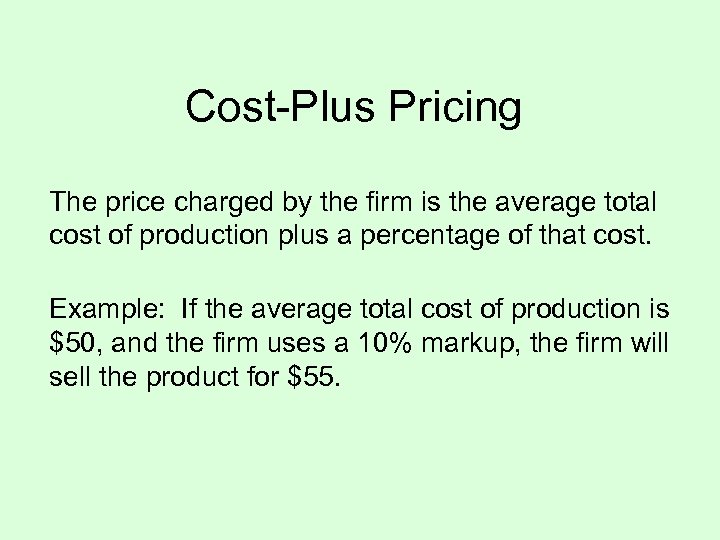Cost-Plus Pricing The price charged by the firm is the average total cost of production plus a percentage of that cost. Example: If the average total cost of production is $50, and the firm uses a 10% markup, the firm will sell the product for $55.

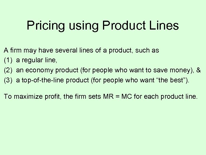Pricing using Product Lines A firm may have several lines of a product, such as (1) a regular line, (2) an economy product (for people who want to save money), & (3) a top-of-the-line product (for people who want “the best”). To maximize profit, the firm sets MR = MC for each product line.

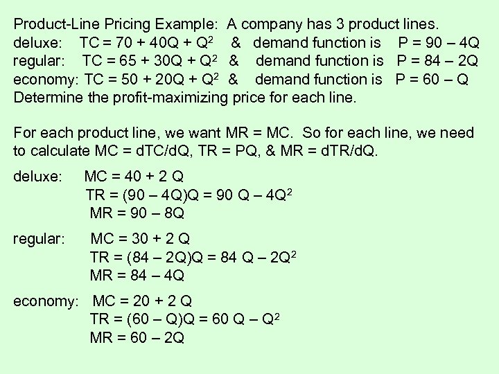Product-Line Pricing Example: A company has 3 product lines. deluxe: TC = 70 + 40 Q + Q 2 & demand function is P = 90 – 4 Q regular: TC = 65 + 30 Q + Q 2 & demand function is P = 84 – 2 Q economy: TC = 50 + 20 Q + Q 2 & demand function is P = 60 – Q Determine the profit-maximizing price for each line. For each product line, we want MR = MC. So for each line, we need to calculate MC = d. TC/d. Q, TR = PQ, & MR = d. TR/d. Q. deluxe: MC = 40 + 2 Q TR = (90 – 4 Q)Q = 90 Q – 4 Q 2 MR = 90 – 8 Q regular: MC = 30 + 2 Q TR = (84 – 2 Q)Q = 84 Q – 2 Q 2 MR = 84 – 4 Q economy: MC = 20 + 2 Q TR = (60 – Q)Q = 60 Q – Q 2 MR = 60 – 2 Q

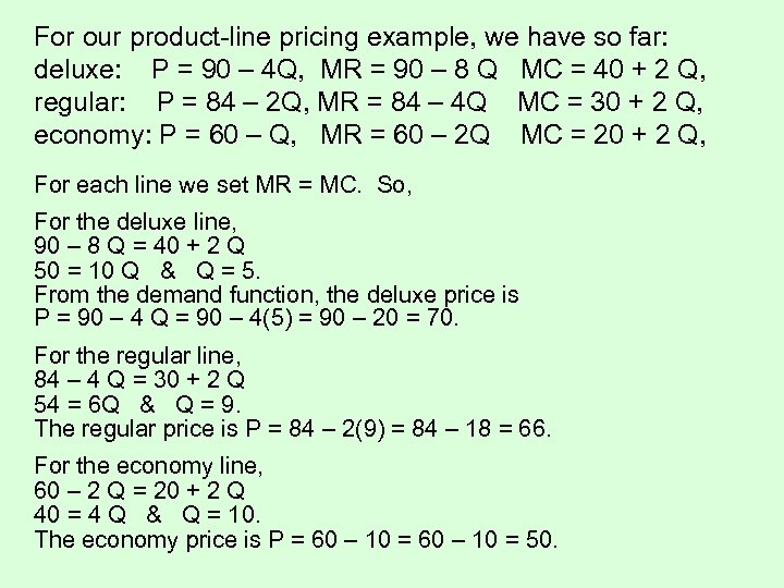For our product-line pricing example, we have so far: deluxe: P = 90 – 4 Q, MR = 90 – 8 Q MC = 40 + 2 Q, regular: P = 84 – 2 Q, MR = 84 – 4 Q MC = 30 + 2 Q, economy: P = 60 – Q, MR = 60 – 2 Q MC = 20 + 2 Q, For each line we set MR = MC. So, For the deluxe line, 90 – 8 Q = 40 + 2 Q 50 = 10 Q & Q = 5. From the demand function, the deluxe price is P = 90 – 4 Q = 90 – 4(5) = 90 – 20 = 70. For the regular line, 84 – 4 Q = 30 + 2 Q 54 = 6 Q & Q = 9. The regular price is P = 84 – 2(9) = 84 – 18 = 66. For the economy line, 60 – 2 Q = 20 + 2 Q 40 = 4 Q & Q = 10. The economy price is P = 60 – 10 = 50.

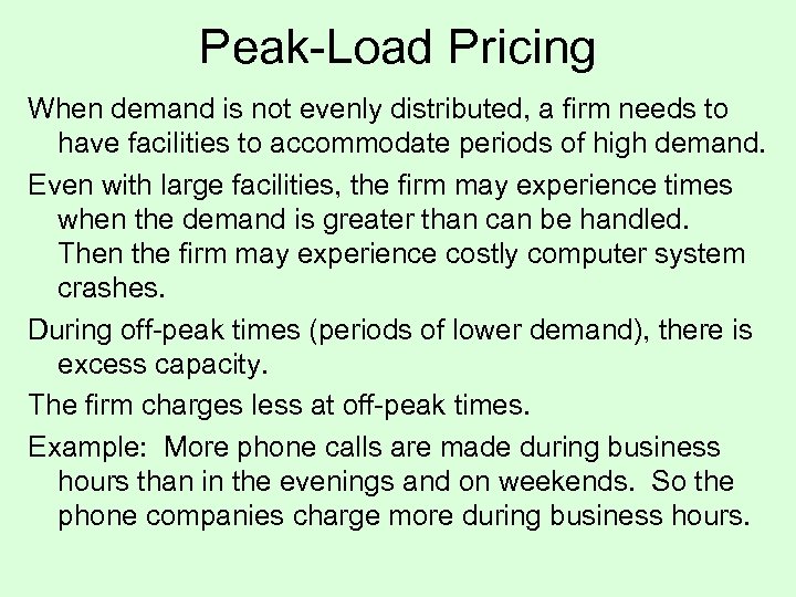Peak-Load Pricing When demand is not evenly distributed, a firm needs to have facilities to accommodate periods of high demand. Even with large facilities, the firm may experience times when the demand is greater than can be handled. Then the firm may experience costly computer system crashes. During off-peak times (periods of lower demand), there is excess capacity. The firm charges less at off-peak times. Example: More phone calls are made during business hours than in the evenings and on weekends. So the phone companies charge more during business hours.

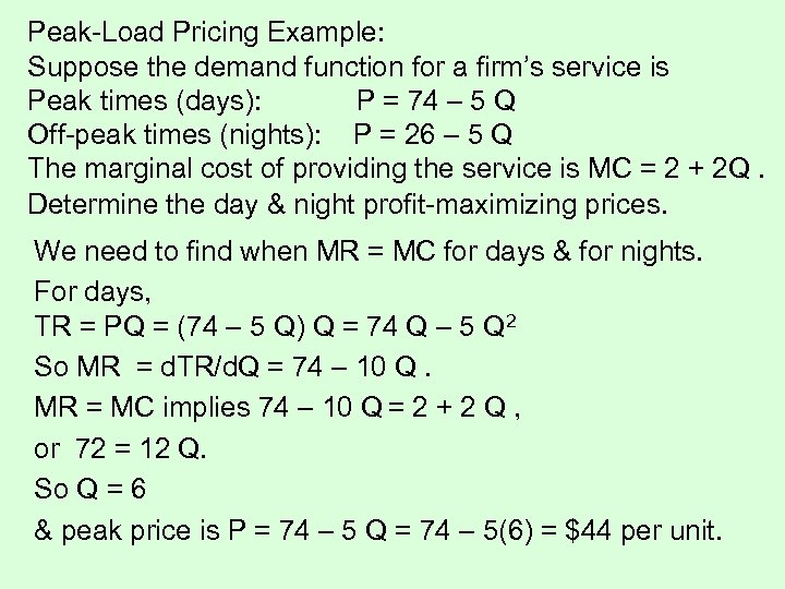Peak-Load Pricing Example: Suppose the demand function for a firm’s service is Peak times (days): P = 74 – 5 Q Off-peak times (nights): P = 26 – 5 Q The marginal cost of providing the service is MC = 2 + 2 Q. Determine the day & night profit-maximizing prices. We need to find when MR = MC for days & for nights. For days, TR = PQ = (74 – 5 Q) Q = 74 Q – 5 Q 2 So MR = d. TR/d. Q = 74 – 10 Q. MR = MC implies 74 – 10 Q = 2 + 2 Q , or 72 = 12 Q. So Q = 6 & peak price is P = 74 – 5 Q = 74 – 5(6) = $44 per unit.

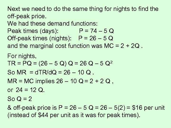Next we need to do the same thing for nights to find the off-peak price. We had these demand functions: Peak times (days): P = 74 – 5 Q Off-peak times (nights): P = 26 – 5 Q and the marginal cost function was MC = 2 + 2 Q. For nights, TR = PQ = (26 – 5 Q) Q = 26 Q – 5 Q 2 So MR = d. TR/d. Q = 26 – 10 Q. MR = MC implies 26 – 10 Q = 2 + 2 Q , or 24 = 12 Q. So Q = 2 & off-peak price is P = 26 – 5 Q = 26 – 5(2) = $16 per unit (instead of $44 per unit as it was for peak times).

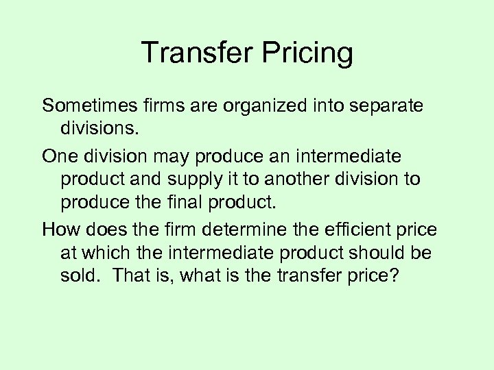Transfer Pricing Sometimes firms are organized into separate divisions. One division may produce an intermediate product and supply it to another division to produce the final product. How does the firm determine the efficient price at which the intermediate product should be sold. That is, what is the transfer price?

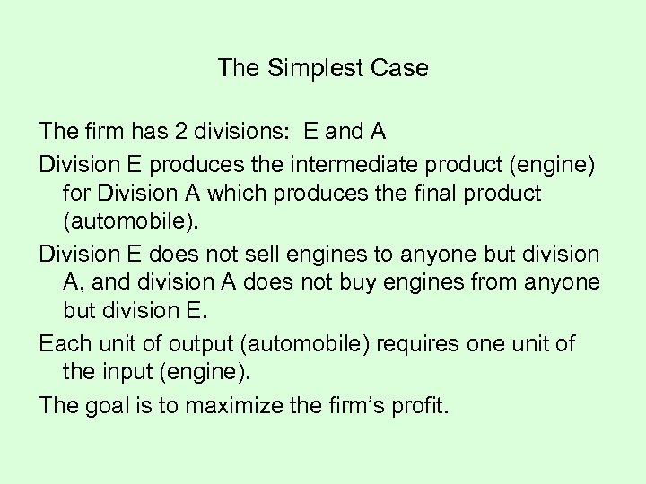The Simplest Case The firm has 2 divisions: E and A Division E produces the intermediate product (engine) for Division A which produces the final product (automobile). Division E does not sell engines to anyone but division A, and division A does not buy engines from anyone but division E. Each unit of output (automobile) requires one unit of the input (engine). The goal is to maximize the firm’s profit.

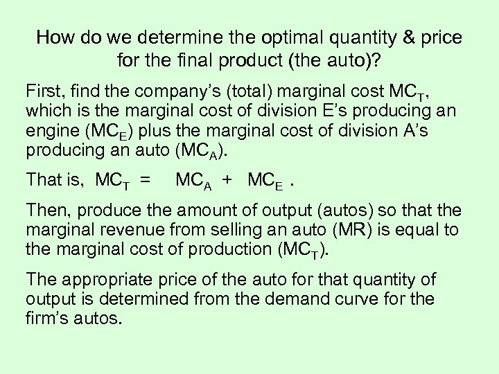How do we determine the optimal quantity & price for the final product (the auto)? First, find the company’s (total) marginal cost MCT, which is the marginal cost of division E’s producing an engine (MCE) plus the marginal cost of division A’s producing an auto (MCA). That is, MCT = MCA + MCE. Then, produce the amount of output (autos) so that the marginal revenue from selling an auto (MR) is equal to the marginal cost of production (MCT). The appropriate price of the auto for that quantity of output is determined from the demand curve for the firm’s autos.

So what is the transfer price at which division E sells the intermediate product to division A? If the company determines the price of the engine, then division E is a price taker. So, PE and MRE will be equal. The firm should set the price of the intermediate product (the engine) so that PE = MRE = MCE at the profit-maximizing output level previously determined.

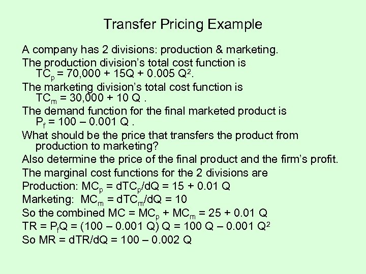Transfer Pricing Example A company has 2 divisions: production & marketing. The production division’s total cost function is TCp = 70, 000 + 15 Q + 0. 005 Q 2. The marketing division’s total cost function is TCm = 30, 000 + 10 Q. The demand function for the final marketed product is Pf = 100 – 0. 001 Q. What should be the price that transfers the product from production to marketing? Also determine the price of the final product and the firm’s profit. The marginal cost functions for the 2 divisions are Production: MCp = d. TCp/d. Q = 15 + 0. 01 Q Marketing: MCm = d. TCm/d. Q = 10 So the combined MC = MCp + MCm = 25 + 0. 01 Q TR = Pf. Q = (100 – 0. 001 Q) Q = 100 Q – 0. 001 Q 2 So MR = d. TR/d. Q = 100 – 0. 002 Q

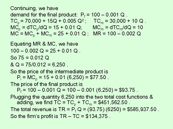Continuing, we have demand for the final product: Pf = 100 – 0. 001 Q. TCp = 70, 000 + 15 Q + 0. 005 Q 2 ; TCm = 30, 000 + 10 Q. MCp = d. TCp/d. Q = 15 + 0. 01 Q; MCm = d. TCm/d. Q = 10 MC = MCp + MCm = 25 + 0. 01 Q ; MR = 100 – 0. 002 Q Equating MR & MC, we have 100 – 0. 002 Q = 25 + 0. 01 Q. So 75 = 0. 012 Q & Q = 75/0. 012 = 6, 250. So the price of the intermediate product is Pi = MCp = 15 + 0. 01 (6, 250) = $77. 50. The price of the final product is Pf = 100 – 0. 001 Q = 100 – 0. 001 (6, 250) = $93. 75. Plugging the quantity 6, 250 into the two total cost functions & adding, we find TC = TCp + TCm = $451, 562. 50. The total revenue is TR = Pf Q = (93. 75) (6250) = $585, 937. 50. So the firm’s profit is TR – TC = $134, 375.