Pricing Strategies Pricing and Profits 8

Pricing Strategies

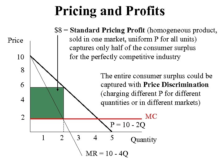Pricing and Profits $8 = Standard Pricing Profit (homogeneous product, sold in one market, uniform P for all units) captures only half of the consumer surplus for the perfectly competitive industry Price 10 8 The entire consumer surplus could be captured with Price Discrimination (charging different P for different quantities or in different markets) 6 4 MC 2 P = 10 - 2 Q 1 2 3 4 5 MR = 10 - 4 Q Quantity

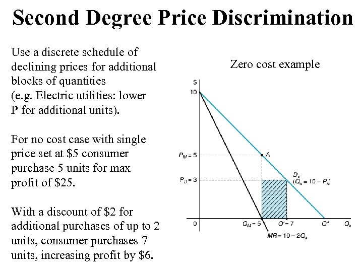Second Degree Price Discrimination Use a discrete schedule of declining prices for additional blocks of quantities (e. g. Electric utilities: lower P for additional units). For no cost case with single price set at $5 consumer purchase 5 units for max profit of $25. With a discount of $2 for additional purchases of up to 2 units, consumer purchases 7 units, increasing profit by $6. Zero cost example

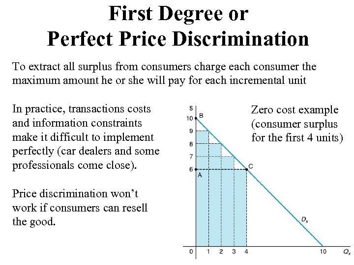First Degree or Perfect Price Discrimination To extract all surplus from consumers charge each consumer the maximum amount he or she will pay for each incremental unit In practice, transactions costs and information constraints make it difficult to implement perfectly (car dealers and some professionals come close). Price discrimination won’t work if consumers can resell the good. Zero cost example (consumer surplus for the first 4 units)

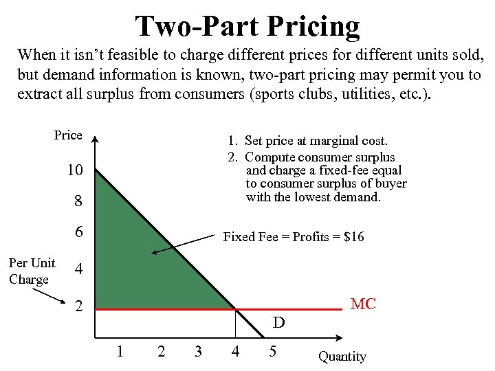Two-Part Pricing When it isn’t feasible to charge different prices for different units sold, but demand information is known, two-part pricing may permit you to extract all surplus from consumers (sports clubs, utilities, etc. ). Price 8 1. Set price at marginal cost. 2. Compute consumer surplus and charge a fixed-fee equal to consumer surplus of buyer with the lowest demand. 6 Fixed Fee = Profits = $16 10 Per Unit Charge 4 MC 2 D 1 2 3 4 5 Quantity

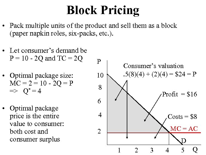Block Pricing • Pack multiple units of the product and sell them as a block (paper napkin roles, six-packs, etc. ). • Let consumer’s demand be P = 10 - 2 Q and TC = 2 Q • Optimal package size: MC = 2 = 10 - 2 Q = P => Q* = 4 • Optimal package price is the entire value to consumer: both cost and consumer surplus P Consumer’s valuation. 5(8)(4) + (2)(4) = $24 = P 10 8 Profit = $16 6 4 Costs = $8 2 MC = AC 1 2 3 4 D 5 Q

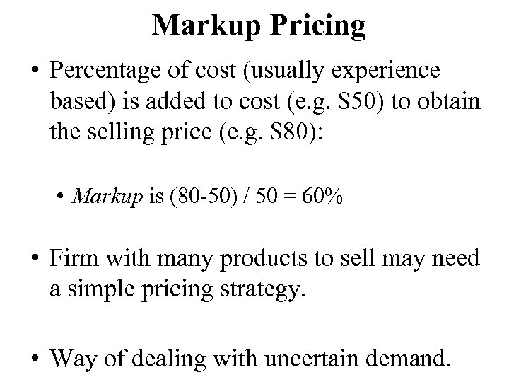Markup Pricing • Percentage of cost (usually experience based) is added to cost (e. g. $50) to obtain the selling price (e. g. $80): • Markup is (80 -50) / 50 = 60% • Firm with many products to sell may need a simple pricing strategy. • Way of dealing with uncertain demand.

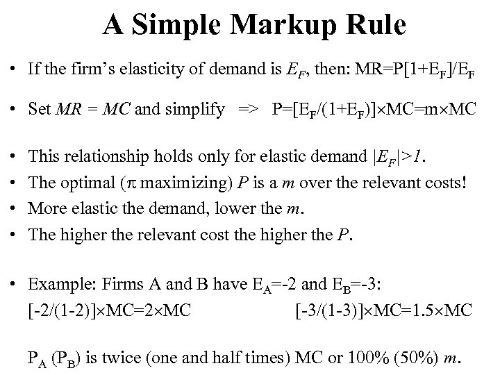A Simple Markup Rule • If the firm’s elasticity of demand is EF, then: MR=P[1+EF]/EF • Set MR = MC and simplify => P=[EF/(1+EF)] MC=m MC • • This relationship holds only for elastic demand |EF|>1. The optimal ( maximizing) P is a m over the relevant costs! More elastic the demand, lower the m. The higher the relevant cost the higher the P. • Example: Firms A and B have EA=-2 and EB=-3: [-2/(1 -2)] MC=2 MC [-3/(1 -3)] MC=1. 5 MC PA (PB) is twice (one and half times) MC or 100% (50%) m.

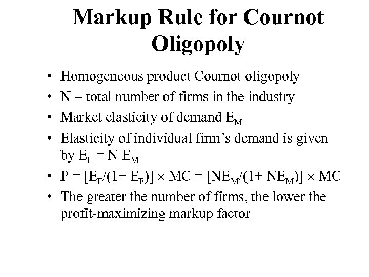Markup Rule for Cournot Oligopoly • • Homogeneous product Cournot oligopoly N = total number of firms in the industry Market elasticity of demand EM Elasticity of individual firm’s demand is given by EF = N EM • P = [EF/(1+ EF)] MC = [NEM/(1+ NEM)] MC • The greater the number of firms, the lower the profit-maximizing markup factor

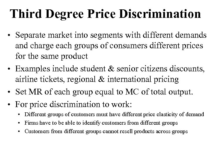Third Degree Price Discrimination • Separate market into segments with different demands and charge each groups of consumers different prices for the same product • Examples include student & senior citizens discounts, airline tickets, regional & international pricing • Set MR of each group equal to MC of total output. • For price discrimination to work: • Different groups of customers must have different price elasticity of demand • Firms have to be able to identify customers from different groups • Customers from different groups cannot resell products across groups

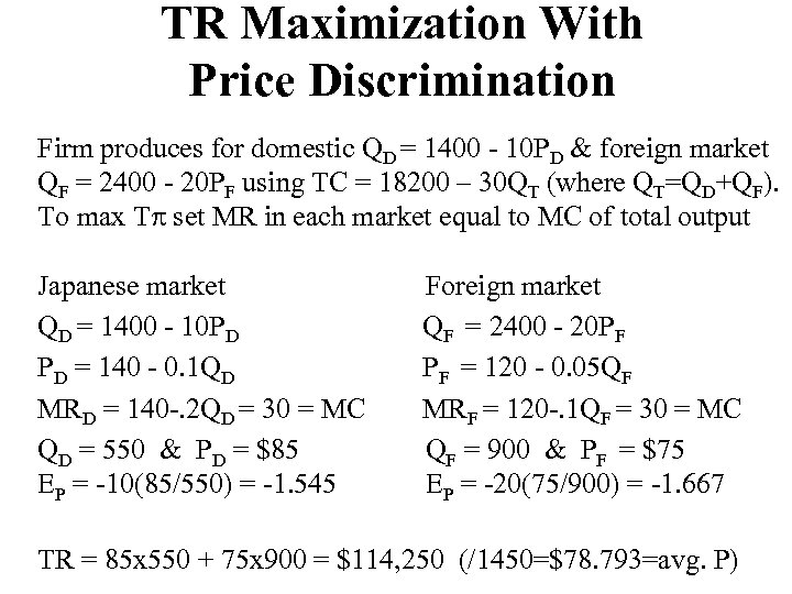TR Maximization With Price Discrimination Firm produces for domestic QD = 1400 - 10 PD & foreign market QF = 2400 - 20 PF using TC = 18200 – 30 QT (where QT=QD+QF). To max T set MR in each market equal to MC of total output Japanese market QD = 1400 - 10 PD PD = 140 - 0. 1 QD MRD = 140 -. 2 QD = 30 = MC QD = 550 & PD = $85 EP = -10(85/550) = -1. 545 Foreign market QF = 2400 - 20 PF PF = 120 - 0. 05 QF MRF = 120 -. 1 QF = 30 = MC QF = 900 & PF = $75 EP = -20(75/900) = -1. 667 TR = 85 x 550 + 75 x 900 = $114, 250 (/1450=$78. 793=avg. P)

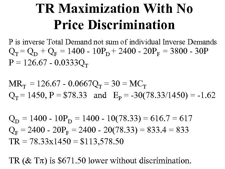TR Maximization With No Price Discrimination P is inverse Total Demand not sum of individual Inverse Demands QT = QD + QF = 1400 - 10 PD + 2400 - 20 PF = 3800 - 30 P P = 126. 67 - 0. 0333 QT MRT = 126. 67 - 0. 0667 QT = 30 = MCT QT = 1450, P = $78. 33 and EP = -30(78. 33/1450) = -1. 62 QD = 1400 - 10 PD = 1400 - 10(78. 33) = 616. 7 = 617 QF = 2400 - 20 PF = 2400 - 20(78. 33) = 833. 4 = 833 TR = 78. 33 x 1450 = $113, 578. 50 TR (& T ) is $671. 50 lower without discrimination.

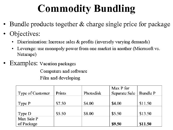Commodity Bundling • Bundle products together & charge single price for package • Objectives: • Discrimination: Increase sales & profits (inversely varying demands) • Leverage: use monopoly power from one market in another (Microsoft vs. Netscape) • Examples: Vacation packages Computers and software Film and developing

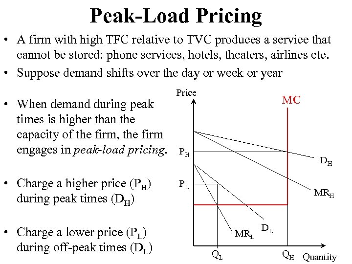Peak-Load Pricing • A firm with high TFC relative to TVC produces a service that cannot be stored: phone services, hotels, theaters, airlines etc. • Suppose demand shifts over the day or week or year • When demand during peak times is higher than the capacity of the firm, the firm engages in peak-load pricing. • Charge a higher price (PH) during peak times (DH) • Charge a lower price (PL) during off-peak times (DL) Price MC PH DH PL MRH MRL QL DL QH Quantity

Cross-Subsidies • Prices charged for one product are subsidized by the sale of another product • May be profitable when there are significant demand complementarities effects • Examples • Browser and server software • Drinks and meals at restaurants

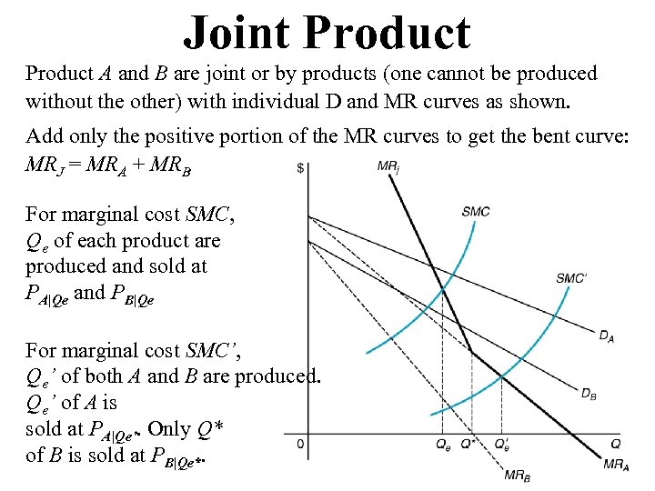Joint Product A and B are joint or by products (one cannot be produced without the other) with individual D and MR curves as shown. Add only the positive portion of the MR curves to get the bent curve: MRJ = MRA + MRB For marginal cost SMC, Qe of each product are produced and sold at PA|Qe and PB|Qe For marginal cost SMC’, Qe’ of both A and B are produced. Qe’ of A is sold at PA|Qe’. Only Q* of B is sold at PB|Qe*.

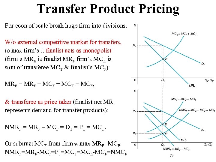Transfer Product Pricing For econ of scale break huge firm into divisions. W/o external competitive market for transfers, to max firm’s finalist acts as monopolist (firm’s MRE is finalist MRF firm’s MCE is sum of transferee MCT & finalist’s MCF): MRE = MRF = MCF + MCT = MCE, & transferee as price taker (finalist net MR represents demand for transfer products): NMRF = MRF – MCF = DT = PT = MCT. Or subtract MCF from firm max MRF=MCE: NMRF=MRF-MCF=PT=MCE-MCF=NMCF

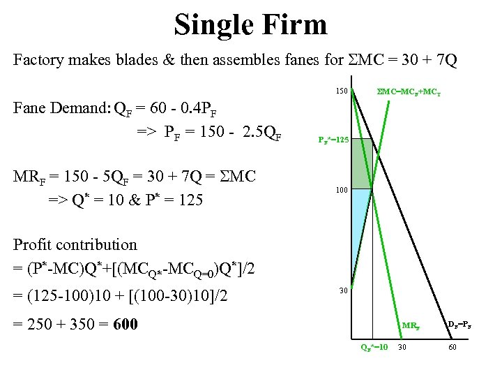Single Firm Factory makes blades & then assembles fanes for MC = 30 + 7 Q 150 Fane Demand: QF = 60 - 0. 4 PF => PF = 150 - 2. 5 QF MRF = 150 - 5 QF = 30 + 7 Q = MC => Q* = 10 & P* = 125 MC=MCF+MCT PF*=125 100 Profit contribution = (P*-MC)Q*+[(MCQ*-MCQ=0)Q*]/2 = (125 -100)10 + [(100 -30)10]/2 30 = 250 + 350 = 600 MRF QF*=10 30 DF=PF 60

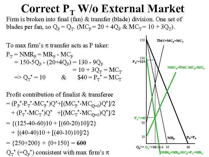Correct PT W/o External Market Firm is broken into final (fan) & transfer (blade) division. One set of blades per fan, so QF = QT. (MCF = 20 + 4 QF & MCT = 10 + 3 QT). To max firm’s transfer acts as P taker: PT = NMRF = MRF - MCF = 150 -5 QF - (20+4 QF) = 130 - 9 QF = 10 + 3 QT = MCT => QT* = 10 & $40 = PT* = MCT Profit contribution of finalist & transferee = (PF*-PT*-MCF*)Q*+[(MCF*-MCQ=0)Q*]/2 + (PT*-MCT*)Q* +[(MCT*-MCQ=0)Q*]/2 = {(125 -40 -60)10 + [(60 -20)10]/2} + {(40 -40)10 + [(40 -10)10]/2} = {250+200} + {0+150} = 600 QT* (=QF*) consistent with max firm’s 150 MC=MCF+MCT 130 PF*=125 NMCF= MC-MCF=MCT PT*=40 30 10 MRF DF=PF QF*= QT*=10 14. 4 30 60 NMRF=MRF-MCF=PT=MRT

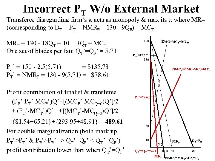Incorrect PT W/o External Market Transferee disregarding firm’s acts as monopoly & max its where MRT (corresponding to DT = PT = NMRF = 130 - 9 QF) = MCT: MRT = 130 - 18 QT = 10 + 3 QT = MCT One set of blades per fan: QT’=QF’ = 5. 71 150 MC=MCF+MCT PF’=135. 73 130 PF’ = 150 - 2. 5(5. 71) = $135. 73 PT’ = NMRF = 130 - 9(5. 71) = $78. 61 Profit contribution of finalist & transferee = (PF’-PT’-MCF’)Q’+[(MCF’-MCQ=0)Q’]/2 + (PT’-MCT’)Q’ +[(MCT’-MCQ=0)Q’]/2 = {81. 54+65. 21}+{293. 95+48. 91} = 489. 61 For double marginalization (both mark up: PT’>PT* & PF’>PF* => QT’=QF’ < QT*=QF*) profit contribution lower than when QT*=QF* NMCF= MC-MCF=MCT PT’=78. 61 30 10 7. 2 MRF DF=PF QF’=QT’=5. 71 14. 4 30 60 MRT NMR =MR -MC =P F F F T

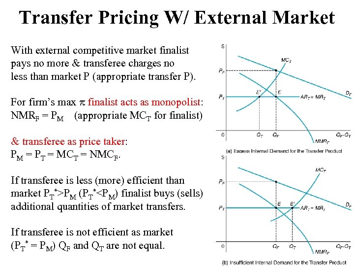Transfer Pricing W/ External Market With external competitive market finalist pays no more & transferee charges no less than market P (appropriate transfer P). For firm’s max finalist acts as monopolist: NMRF = PM (appropriate MCT for finalist) & transferee as price taker: PM = PT = MCT = NMCF. If transferee is less (more) efficient than market PT*>PM (PT*

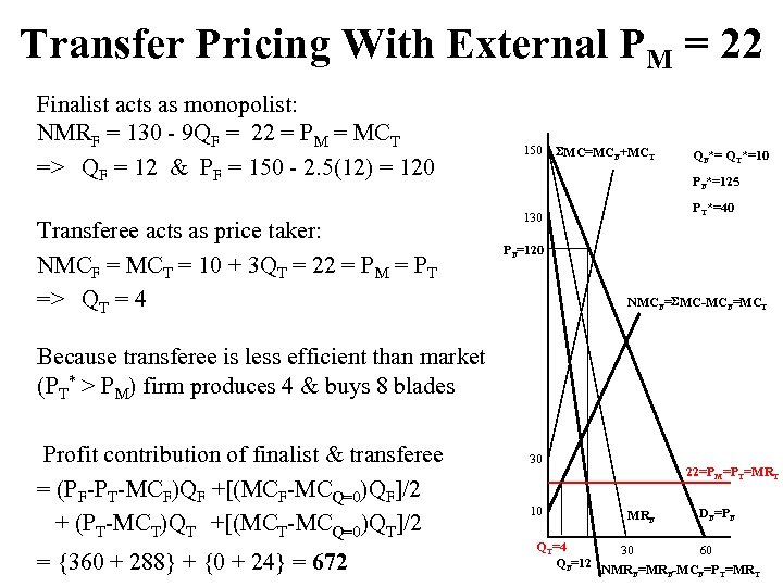Transfer Pricing With External PM = 22 Finalist acts as monopolist: NMRF = 130 - 9 QF = 22 = PM = MCT => QF = 12 & PF = 150 - 2. 5(12) = 120 Transferee acts as price taker: NMCF = MCT = 10 + 3 QT = 22 = PM = PT => QT = 4 150 MC=MCF+MCT QF*= QT*=10 PF*=125 PT*=40 130 PF=120 NMCF= MC-MCF=MCT Because transferee is less efficient than market (PT* > PM) firm produces 4 & buys 8 blades Profit contribution of finalist & transferee = (PF-PT-MCF)QF +[(MCF-MCQ=0)QF]/2 + (PT-MCT)QT +[(MCT-MCQ=0)QT]/2 = {360 + 288} + {0 + 24} = 672 30 10 22=PM=PT=MRT MRF DF=PF QT=4 30 60 QF=12 NMR =MR -MC =P =MR F F F T T

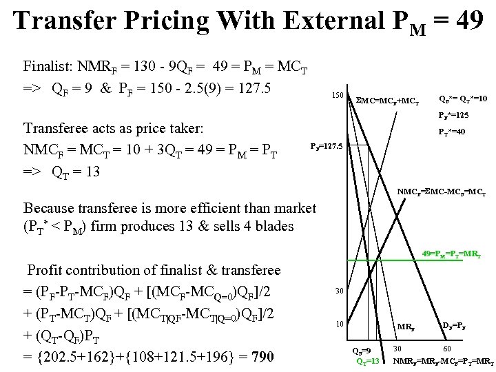Transfer Pricing With External PM = 49 Finalist: NMRF = 130 - 9 QF = 49 = PM = MCT => QF = 9 & PF = 150 - 2. 5(9) = 127. 5 Transferee acts as price taker: NMCF = MCT = 10 + 3 QT = 49 = PM = PT => QT = 13 150 MC=MCF+MCT QF*= QT*=10 PF*=125 PT*=40 PF=127. 5 NMCF= MC-MCF=MCT Because transferee is more efficient than market (PT* < PM) firm produces 13 & sells 4 blades 49=PM=PT=MRT Profit contribution of finalist & transferee = (PF-PT-MCF)QF + [(MCF-MCQ=0)QF]/2 + (PT-MCT)QF + [(MCT|QF-MCT|Q=0)QF]/2 + (QT-QF)PT = {202. 5+162}+{108+121. 5+196} = 790 30 10 MRF QF=9 QT=13 DF=PF 30 60 NMRF=MRF-MCF=PT=MRT

Pricing in Markets with Intense Price Competition Prevent customers to become informed about prices through: • Price Matching • Advertising a price and a promise to match any lower price offered by a competitor. • No firm has an incentive to lower their prices. • Each firm charges the monopoly price and shares the market. • Randomized Pricing • A strategy of constantly changing prices. • Decreases consumers’ incentive to shop around as they cannot learn from experience which firm charges the lowest price. • Reduces the ability of rival firms to undercut a firm’s prices. • Build Brand Loyalty

Recap of Pricing Strategies • First degree price discrimination, block pricing, and two part pricing permit a firm to extract all consumer surplus. • Commodity bundling, second-degree and third degree price discrimination permit a firm to extract some (but not all) consumer surplus. • Simple markup rules are the easiest to implement, but leave consumers with the most surplus and may result in double-marginalization. • Different strategies require different information.