Pricing MKT 6301 Nanda Kumar http www utdallas

Pricing MKT 6301 Nanda Kumar http: //www. utdallas. edu/~nkumar

P&G and EDLP n In 1992, P&G decided to move from Hi-Lo Pricing to EDLP – “Value Pricing” n Achieved this by lowering wholesale list prices by 10 -25% n Motivation – trade promotion spending had gotten out of hand n 44% of all marketing dollars spent on trade promotions compared to 24% a decade earlier

Brand Erosion n Manufacturers had to rely on price- oriented promotions to differentiate their brands n Wholesalers/Retailers expected these price discounts n Consumers had become “deal” loyal instead of “brand” loyal

Other Issues n Retailer Forward Buying n Inventory problems n Demand fluctuations n Supply side inefficiencies

Nature of Conflict n P&G adopted value pricing to restore brand loyalty n Retailers’ resistance n Used promotions to build store traffic (attract value-minded customers) n Often pocketed trade promotion dollars n No longer had control of promotional dollars

Risky Strategy n Reaction of the Trade – Every Day Low Profits! n A&P, Safeway and Rite Aid eliminated selected P&G sizes and dropped marginal brands n Certified Grocers dropped 50 of 300 P&G brands it carried n Other retailers moved P&G from premium eye-level space to less visible shelves n P&G decided to stay the course despite initial drop in sales and market shares Claims the new pricing scheme saves customers over $6 Billion n P&G’s products in most categories are growing steadily and producing healthier profits n

Take Away? n Prices should reflect and enhance the value offered to consumers n Complicated decision even in a direct channel n More complicated with n Intermediaries n Competition

Value-Based Pricing Economic Value Analysis n Assessing what value your customers place on the product or service n Set price less than EV > Price > Cost

How to assess Economic Value? n Economic Value-In-Use n Market research n Conjoint Analysis n Logit Model n Employees with direct customer contact n Sales force

Determining Economic Value-In-Use n Economic Value = Reference Value + Differentiation Value n Reference Value: Price of the best substitute n RV = Price of Competing product adjusted for any difference in quantity used n Differentiation Value: Value of product attributes that are different from those of the best substitute n DV = Positive if customer likes differentiating attribute, Negative otherwise

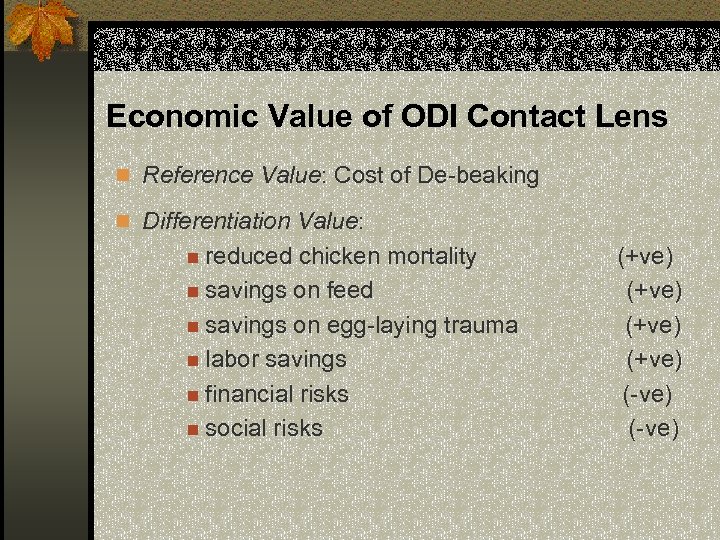Economic Value of ODI Contact Lens n Reference Value: Cost of De-beaking n Differentiation Value: n reduced chicken mortality n savings on feed n savings on egg-laying trauma n labor savings n financial risks n social risks (+ve) (-ve)

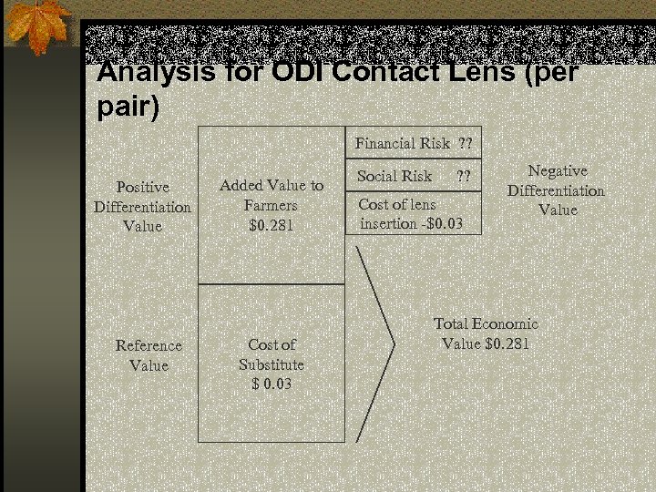Analysis for ODI Contact Lens (per pair) Financial Risk ? ? Positive Differentiation Value Reference Value Added Value to Farmers $0. 281 Cost of Substitute $ 0. 03 Social Risk ? ? Cost of lens insertion -$0. 03 Negative Differentiation Value Total Economic Value $0. 281

Interpreting Economic Value n A product’s market value is determined not only by the economic value but also by the accuracy with which buyers perceive that value n Weakness of EV: Does not indicate the appropriate price to charge. Gives the maximum price consumers will be willing to pay if they were perfectly cognizant of the economic value and were motivated by economic value to make their purchase decisions n Strength of EV: Enables a firm to determine whether a product is selling poorly because it is overpriced relative to its true economic value or because it is under-promoted and consequently, under-appreciated by the market

Other Uses of Economic Value Analysis n Indicates which attribute improvements will result in the greatest n n n enhancement of value Can be used by sales reps to highlight the benefits of the product Help firm identify market segments that value the product’s attributes differently Works well for industrial products and for consumer durables Not very useful for FPP products and for those with “fuzzy” attributes Use methods like Conjoint Analysis

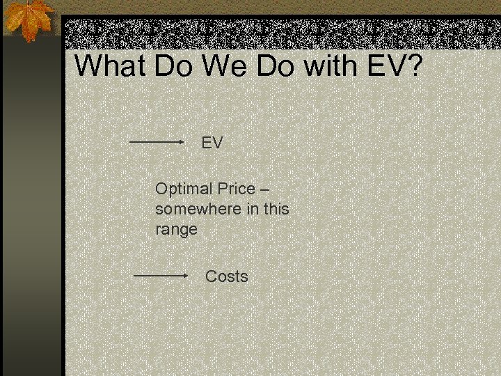What Do We Do with EV? EV Optimal Price – somewhere in this range Costs

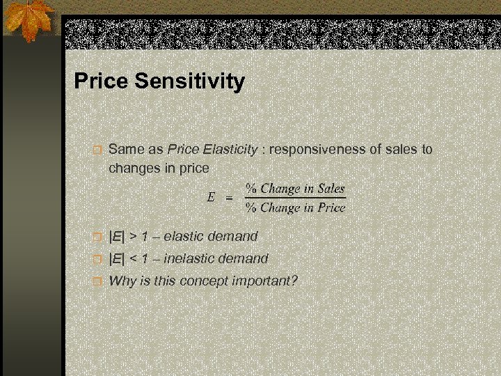Price Sensitivity r Same as Price Elasticity : responsiveness of sales to changes in price r |E| > 1 – elastic demand r |E| < 1 – inelastic demand r Why is this concept important?

Impact of Competition n Market Structure – number of players in the market Monopoly n Oligopoly n Pure Competition n n Competitors’ cost structure n Margins n Lower bound on price

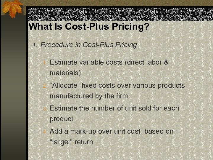What Is Cost-Plus Pricing? 1. Procedure in Cost-Plus Pricing 1. Estimate variable costs (direct labor & materials) 2. “Allocate” fixed costs over various products manufactured by the firm 3. Estimate the number of unit sold for each product 4. Add a mark-up over unit cost, based on “target” return

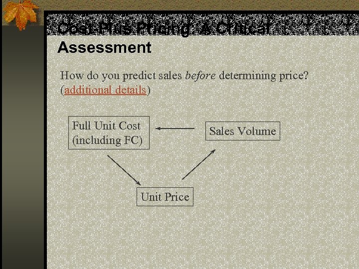Cost-Plus Pricing: A Critical Assessment How do you predict sales before determining price? (additional details) Full Unit Cost (including FC) Unit Price Sales Volume

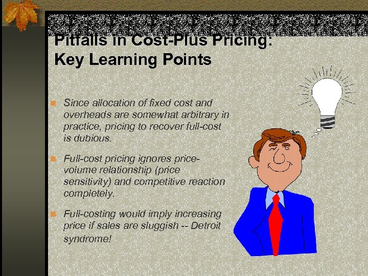Pitfalls in Cost-Plus Pricing: Key Learning Points n Since allocation of fixed cost and overheads are somewhat arbitrary in practice, pricing to recover full-cost is dubious. n Full-cost pricing ignores price- volume relationship (price sensitivity) and competitive reaction completely. n Full-costing would imply increasing price if sales are sluggish -- Detroit syndrome!

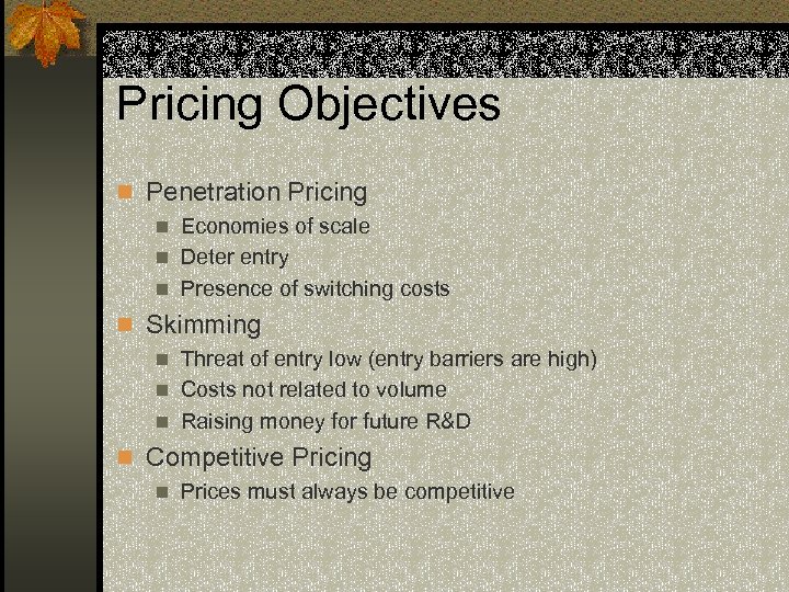Pricing Objectives n Penetration Pricing n Economies of scale n Deter entry n Presence of switching costs n Skimming n Threat of entry low (entry barriers are high) n Costs not related to volume n Raising money for future R&D n Competitive Pricing n Prices must always be competitive

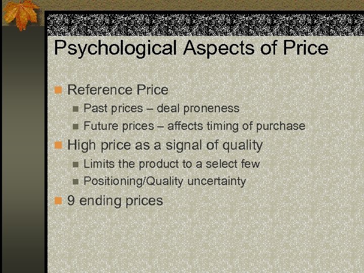Psychological Aspects of Price n Reference Price n Past prices – deal proneness n Future prices – affects timing of purchase n High price as a signal of quality n Limits the product to a select few n Positioning/Quality uncertainty n 9 ending prices

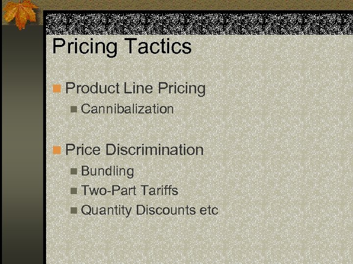Pricing Tactics n Product Line Pricing n Cannibalization n Price Discrimination n Bundling n Two-Part Tariffs n Quantity Discounts etc

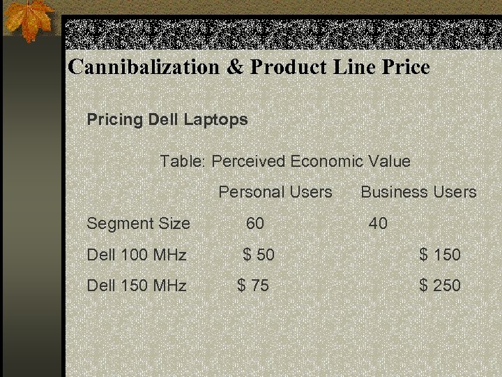Cannibalization & Product Line Pricing Dell Laptops Table: Perceived Economic Value Personal Users Segment Size 60 Dell 100 MHz $ 50 Dell 150 MHz $ 75 Business Users 40 $ 150 $ 250

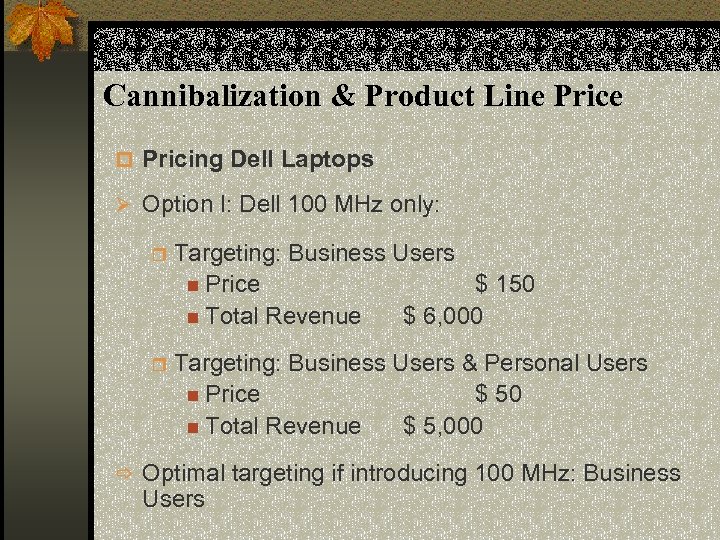Cannibalization & Product Line Price p Pricing Dell Laptops Ø Option I: Dell 100 MHz only: r Targeting: Business Users n Price $ 150 n Total Revenue $ 6, 000 r Targeting: Business Users & Personal Users n Price $ 50 n Total Revenue $ 5, 000 ð Optimal targeting if introducing 100 MHz: Business Users

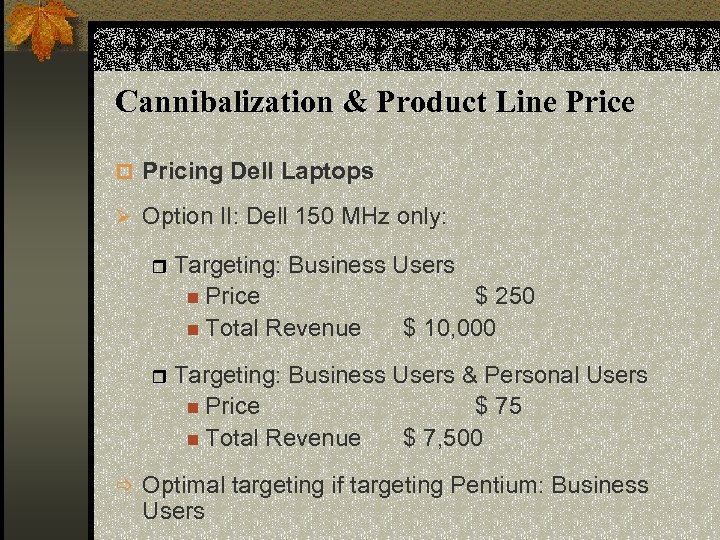Cannibalization & Product Line Price p Pricing Dell Laptops Ø Option II: Dell 150 MHz only: r Targeting: Business Users n Price $ 250 n Total Revenue $ 10, 000 r Targeting: Business Users & Personal Users n Price $ 75 n Total Revenue $ 7, 500 ð Optimal targeting if targeting Pentium: Business Users

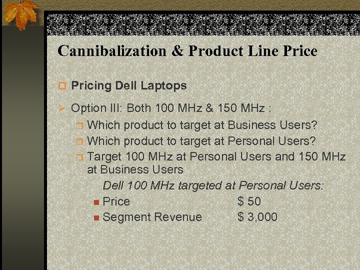Cannibalization & Product Line Price p Pricing Dell Laptops Ø Option III: Both 100 MHz & 150 MHz : Which product to target at Business Users? r Which product to target at Personal Users? r Target 100 MHz at Personal Users and 150 MHz at Business Users Dell 100 MHz targeted at Personal Users: n Price $ 50 n Segment Revenue $ 3, 000 r

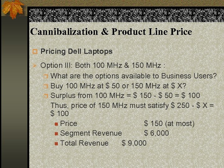Cannibalization & Product Line Price p Pricing Dell Laptops Ø Option III: Both 100 MHz & 150 MHz : What are the options available to Business Users? r Buy 100 MHz at $ 50 or 150 MHz at $ X? r Surplus from 100 MHz = $ 150 - $ 50 = $ 100 Thus, price of 150 MHz must satisfy $ 250 - $ X = $ 100 n Price $ 150 (at most) n Segment Revenue $ 6, 000 n Total Revenue $ 9, 000 r

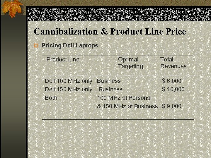Cannibalization & Product Line Price p Pricing Dell Laptops ________________________ Product Line Optimal Total Targeting Revenues ________________________ Dell 100 MHz only Business $ 6, 000 Dell 150 MHz only Business $ 10, 000 Both 100 MHz at Personal & 150 MHz at Business $ 9, 000 ____________________

Product-Line Pricing : Key Learning Points n If price differentials between the items in the product line are not set properly to reflect the variation in EV, profits may decline due to severe cannibalization. n A wider product line is not necessarily a more profitable product line.

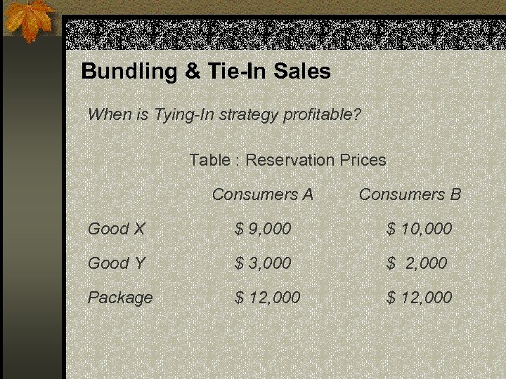Bundling & Tie-In Sales When is Tying-In strategy profitable? Table : Reservation Prices Consumers A Consumers B Good X $ 9, 000 $ 10, 000 Good Y $ 3, 000 $ 2, 000 Package $ 12, 000

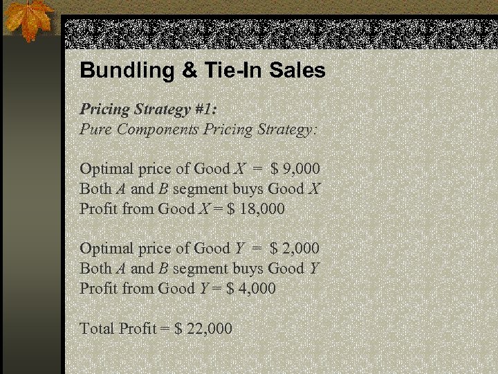Bundling & Tie-In Sales Pricing Strategy #1: Pure Components Pricing Strategy: Optimal price of Good X = $ 9, 000 Both A and B segment buys Good X Profit from Good X = $ 18, 000 Optimal price of Good Y = $ 2, 000 Both A and B segment buys Good Y Profit from Good Y = $ 4, 000 Total Profit = $ 22, 000

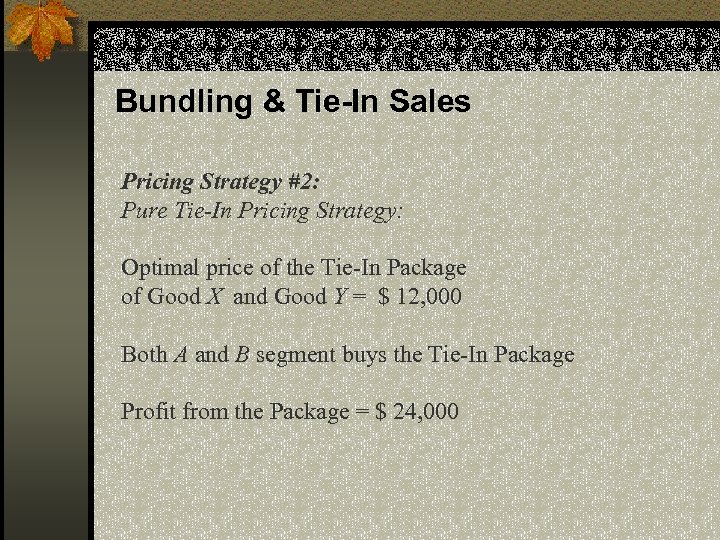Bundling & Tie-In Sales Pricing Strategy #2: Pure Tie-In Pricing Strategy: Optimal price of the Tie-In Package of Good X and Good Y = $ 12, 000 Both A and B segment buys the Tie-In Package Profit from the Package = $ 24, 000

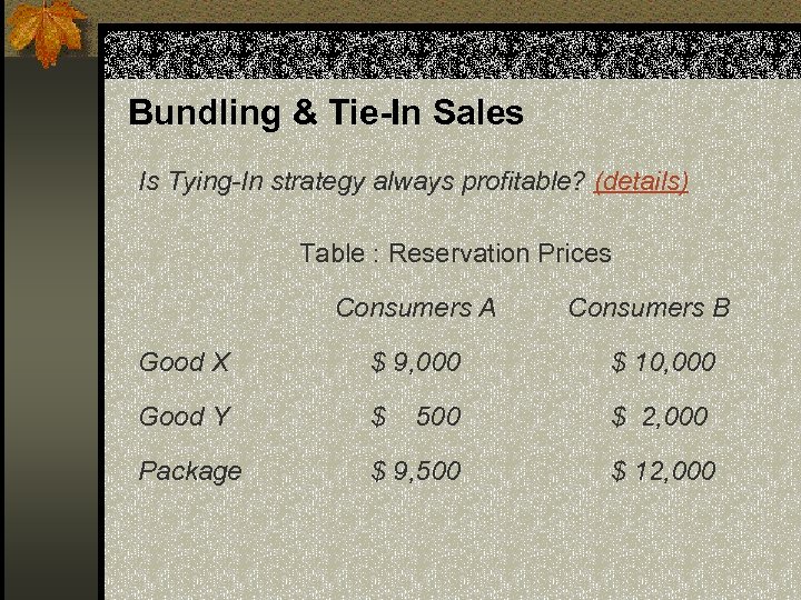Bundling & Tie-In Sales Is Tying-In strategy always profitable? (details) Table : Reservation Prices Consumers A Consumers B Good X $ 9, 000 $ 10, 000 Good Y $ 500 $ 2, 000 Package $ 9, 500 $ 12, 000

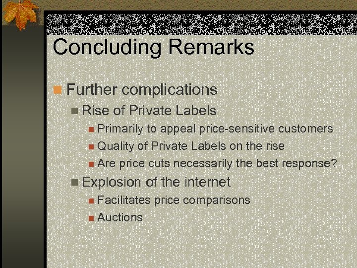Concluding Remarks n Further complications n Rise of Private Labels n Primarily to appeal price-sensitive customers n Quality of Private Labels on the rise n Are price cuts necessarily the best response? n Explosion of the internet n Facilitates n Auctions price comparisons

Pricing Supplemental Notes

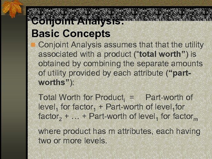Conjoint Analysis: Basic Concepts n Conjoint Analysis assumes that the utility associated with a product (“total worth”) is obtained by combining the separate amounts of utility provided by each attribute (“partworths”): Total Worth for Producti = Part-worth of level 1 for factor 1 + Part-worth of level 1 for factor 2 + … + Part-worth of level 1 for factorm where product has m attributes, each having two or more levels.

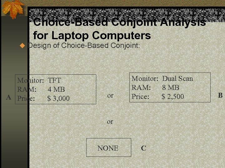Choice-Based Conjoint Analysis for Laptop Computers u Design of Choice-Based Conjoint: Monitor: TFT RAM: 4 MB A Price: $ 3, 000 or Monitor: Dual Scan RAM: 8 MB Price: $ 2, 500 or NONE C B

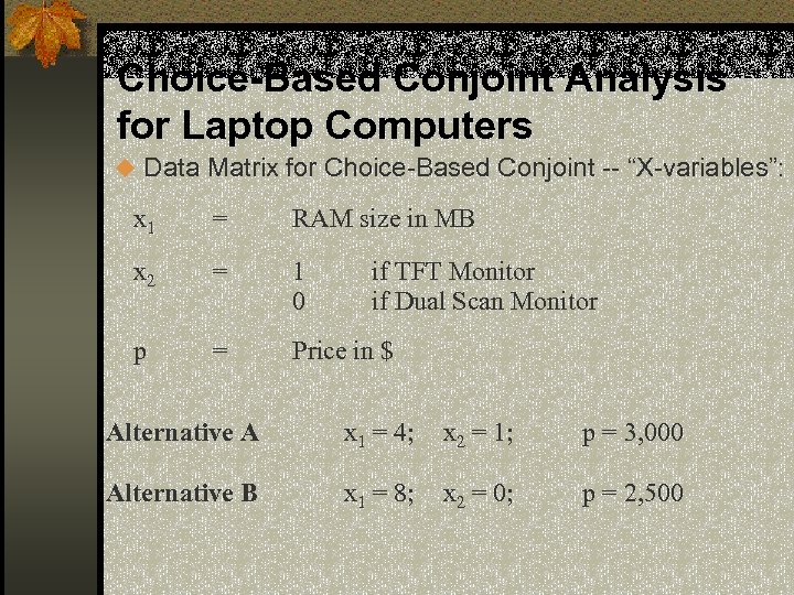Choice-Based Conjoint Analysis for Laptop Computers u Data Matrix for Choice-Based Conjoint -- “X-variables”: x 1 = RAM size in MB x 2 = 1 0 p = Price in $ if TFT Monitor if Dual Scan Monitor Alternative A x 1 = 4; x 2 = 1; p = 3, 000 Alternative B x 1 = 8; x 2 = 0; p = 2, 500

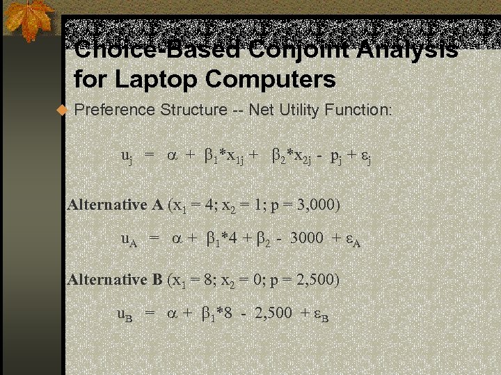Choice-Based Conjoint Analysis for Laptop Computers u Preference Structure -- Net Utility Function: uj = a + b 1*x 1 j + b 2*x 2 j - pj + ej Alternative A (x 1 = 4; x 2 = 1; p = 3, 000) u. A = a + b 1*4 + b 2 - 3000 + e. A Alternative B (x 1 = 8; x 2 = 0; p = 2, 500) u. B = a + b 1*8 - 2, 500 + e. B

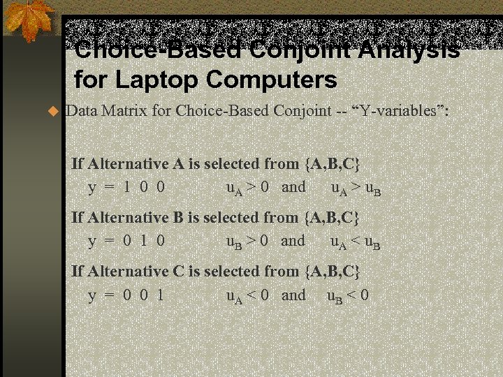Choice-Based Conjoint Analysis for Laptop Computers u Data Matrix for Choice-Based Conjoint -- “Y-variables”: If Alternative A is selected from {A, B, C} y = 1 0 0 u. A > 0 and u. A > u. B If Alternative B is selected from {A, B, C} y = 0 1 0 u. B > 0 and u. A < u. B If Alternative C is selected from {A, B, C} y = 0 0 1 u. A < 0 and u. B < 0

Traditional Conjoint Analysis: Key Learning Point n Multivariate technique n Determine the relative importance consumers attach to salient attributes and the utilities they attach to the levels of attributes n Based on the premise that consumers evaluate the value or utility of a product/service/idea (real or hypothetical) by combining the separate amounts of utility provided by each attribute

Traditional Conjoint Analysis: Key Learning Point 1. Decompositional technique -- respondents evaluate combinations of attributes; CA infers the relative importance and utilities from these evaluations 2. Preferable to asking respondents how important certain attributes are, or to rate how well a product performs on each of a number of attributes (back)

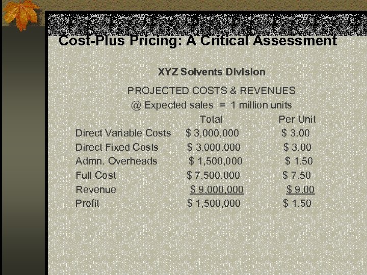Cost-Plus Pricing: A Critical Assessment XYZ Solvents Division PROJECTED COSTS & REVENUES @ Expected sales = 1 million units Total Per Unit Direct Variable Costs $ 3, 000 $ 3. 00 Direct Fixed Costs $ 3, 000 $ 3. 00 Admn. Overheads $ 1, 500, 000 $ 1. 50 Full Cost $ 7, 500, 000 $ 7. 50 Revenue $ 9, 000 $ 9. 00 Profit $ 1, 500, 000 $ 1. 50

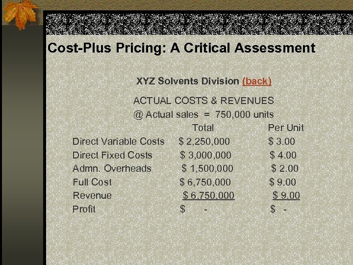Cost-Plus Pricing: A Critical Assessment XYZ Solvents Division (back) ACTUAL COSTS & REVENUES @ Actual sales = 750, 000 units Total Per Unit Direct Variable Costs $ 2, 250, 000 $ 3. 00 Direct Fixed Costs $ 3, 000 $ 4. 00 Admn. Overheads $ 1, 500, 000 $ 2. 00 Full Cost $ 6, 750, 000 $ 9. 00 Revenue $ 6, 750, 000 $ 9. 00 Profit $ $ -

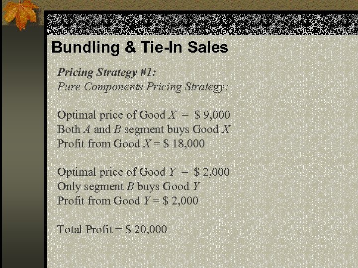Bundling & Tie-In Sales Pricing Strategy #1: Pure Components Pricing Strategy: Optimal price of Good X = $ 9, 000 Both A and B segment buys Good X Profit from Good X = $ 18, 000 Optimal price of Good Y = $ 2, 000 Only segment B buys Good Y Profit from Good Y = $ 2, 000 Total Profit = $ 20, 000

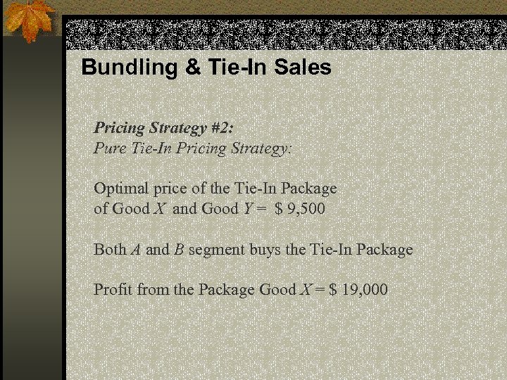Bundling & Tie-In Sales Pricing Strategy #2: Pure Tie-In Pricing Strategy: Optimal price of the Tie-In Package of Good X and Good Y = $ 9, 500 Both A and B segment buys the Tie-In Package Profit from the Package Good X = $ 19, 000

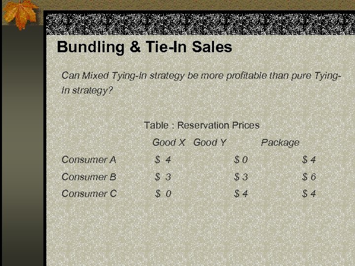Bundling & Tie-In Sales Can Mixed Tying-In strategy be more profitable than pure Tying. In strategy? Table : Reservation Prices Good X Good Y Package Consumer A $ 4 $0 $4 Consumer B $ 3 $3 $6 Consumer C $ 0 $4 $4

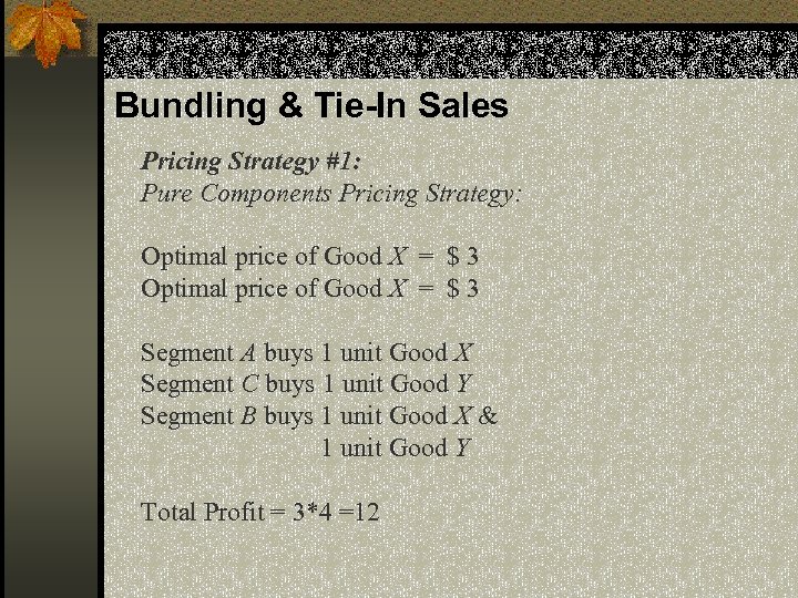Bundling & Tie-In Sales Pricing Strategy #1: Pure Components Pricing Strategy: Optimal price of Good X = $ 3 Segment A buys 1 unit Good X Segment C buys 1 unit Good Y Segment B buys 1 unit Good X & 1 unit Good Y Total Profit = 3*4 =12

Bundling & Tie-In Sales Pricing Strategy #2: Pure Tie-In Pricing Strategy: Optimal price of Package = $ 4 All consumer segments buy the package Total Profit = 3*4 =12

Bundling & Tie-In Sales Pricing Strategy #3: Mixed Tie-In Pricing Strategy: Choice of either a) Package of Good X and Y at $6 b) Individual Goods X and Y at $ 4 each Segment B buys the Package Segment A buys Good X only Segment C buys Y only Total Profit = $ 14

Bundling & Tie-In Sales : Key Learning Points n Tying-In sales is profitable if the preferences of consumers across the various components of the package are negatively correlated. n Gains from tying-in increases with greater degree of negative correlation and/or with larger variation in the valuation of the components

Optimal Tie-In Sales Strategy: Key Learning Points n If customers display similarity in their valuations -- all viewing one product as relatively high value and the other low => Pure Components. n If the markets is characterized by a combination of customers -- both those with “extreme” preferences and those with “balanced” preferences -- seeing the products as equally valuable => Mixed Tie-In Sales back