faaead23660867a3780864ee28b7f87a.ppt
- Количество слайдов: 18
Prices vs. Quantities • Distributional Issues * Baumol and Oates (I believe) • Uncertainty * Weitzman, Martin. “Prices vs. Quantities. ” Review of Economic Studies. Oct 1974 61(4): 477 -491 – Simplify: make benefits deterministic (c) 1998 by Peter Berck
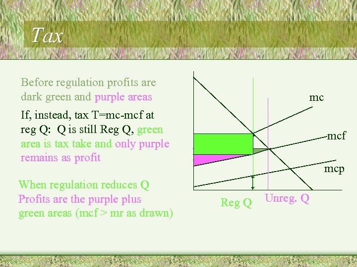
Tax Before regulation profits are dark green and purple areas mc If, instead, tax T=mc-mcf at reg Q: Q is still Reg Q, green area is tax take and only purple remains as profit When regulation reduces Q Profits are the purple plus green areas (mcf > mr as drawn) mcf mcp Reg Q Unreg. Q
The Uncertainty Problem • A private producer needs to be motivated to produce a good that is not sold in a market. • The government does not know the costs of producing the goods. • In particular it does not know a, a mean zero variance 2 element of the cost function
Quantity Regulation • The firm can be told to produce a quantity certain, qr. • The level of benefits will be certain, since qr is certain, but • the level of costs isn’t known so the government will accept the uncertainty in the cost to be paid.
Price Motivation • Or, the Government can offer to pay a price, p for any units produced. * The firm will observe which cost they incur and react to the true supply curve and set p=mc correctly, * but the level of production and level of benefits will be variable
Which to choose? • Professor Weitzman (to the best of my ancient memory) gave the example of medicine to be delivered to wartime Nicaragua. * Too little and people die * Too much not worth anything more * cost doesn’t matter that much * so, choose qr and get the right amount there for certain
In quantity mode, • the regulator chooses a quantity, qr, • then the state of nature becomes known, • then the firm produces and costs are incurred and benefits received. • B(q) is benefits and B’ is marginal benefit. • C(q, a) is cost and is a function of the state of nature, a.
B’ = MC * qr = argmaxq E( B - C). • Gives the optimal choice of qr. • Of course, E[B’ - Cq] = 0 at qr.
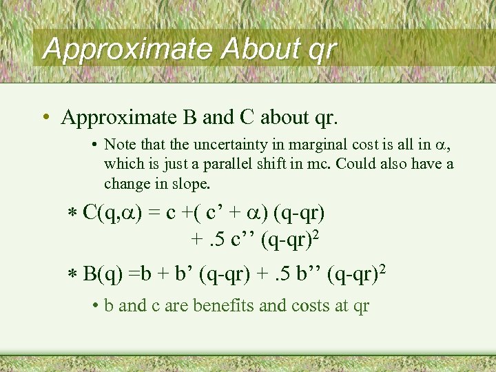
Approximate About qr • Approximate B and C about qr. • Note that the uncertainty in marginal cost is all in a, which is just a parallel shift in mc. Could also have a change in slope. * C(q, a) = c +( c’ + a) (q-qr) +. 5 c’’ (q-qr)2 * B(q) =b + b’ (q-qr) +. 5 b’’ (q-qr)2 • b and c are benefits and costs at qr
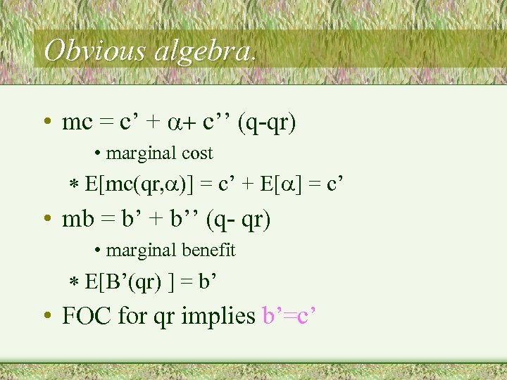
Obvious algebra. • mc = c’ + a+ c’’ (q-qr) • marginal cost * E[mc(qr, a)] = c’ + E[a] = c’ • mb = b’ + b’’ (q- qr) • marginal benefit * E[B’(qr) ] = b’ • FOC for qr implies b’=c’
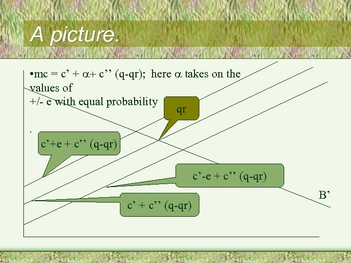
A picture. • mc = c’ + a+ c’’ (q-qr); here a takes on the values of +/- e with equal probability qr. c’+e + c’’ (q-qr) c’-e + c’’ (q-qr) c’ + c’’ (q-qr) B’
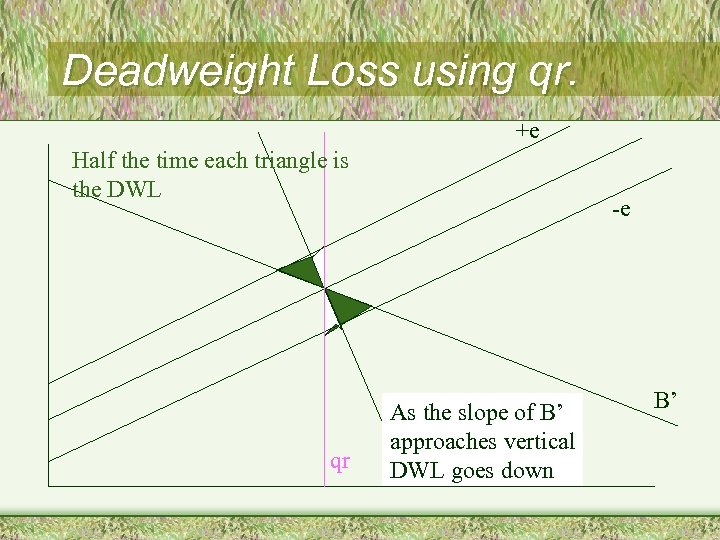
Deadweight Loss using qr. +e Half the time each triangle is the DWL qr -e As the slope of B’ approaches vertical DWL goes down B’
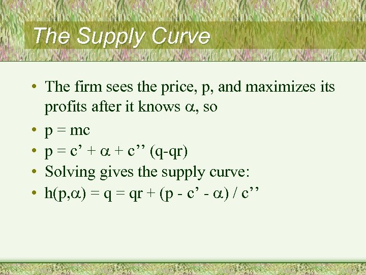
The Supply Curve • The firm sees the price, p, and maximizes its profits after it knows a, so • p = mc • p = c’ + a + c’’ (q-qr) • Solving gives the supply curve: • h(p, a) = qr + (p - c’ - a) / c’’
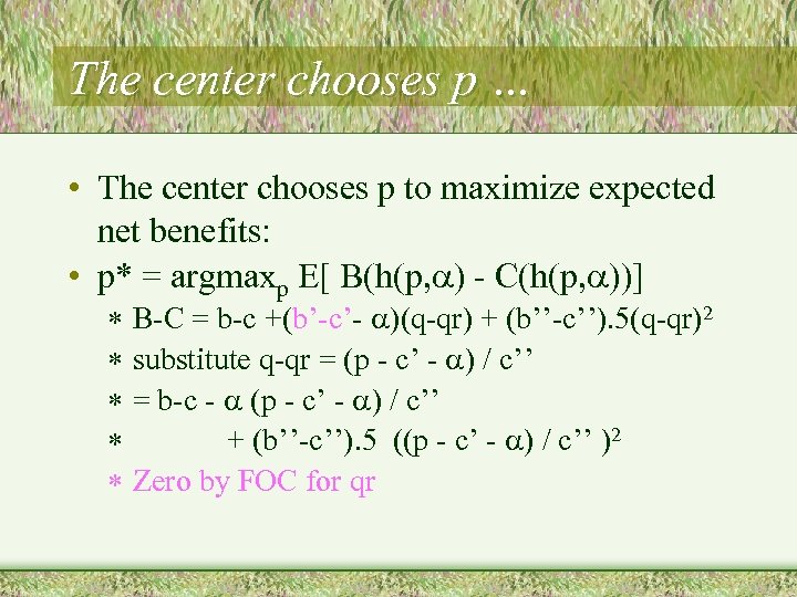
The center chooses p … • The center chooses p to maximize expected net benefits: • p* = argmaxp E[ B(h(p, a) - C(h(p, a))] * B-C = b-c +(b’-c’- a)(q-qr) + (b’’-c’’). 5(q-qr)2 * substitute q-qr = (p - c’ - a) / c’’ * = b-c - a (p - c’ - a) / c’’ * + (b’’-c’’). 5 ((p - c’ - a) / c’’ )2 * Zero by FOC for qr
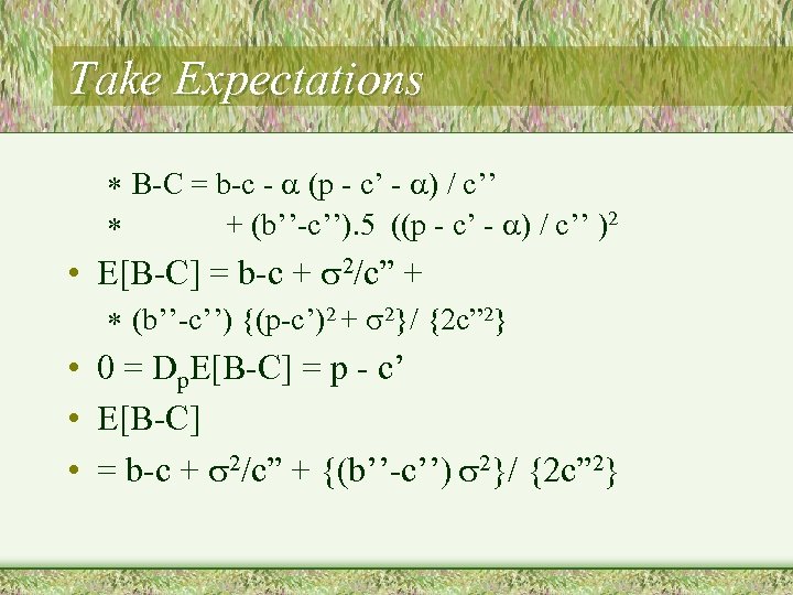
Take Expectations * B-C = b-c - a (p - c’ - a) / c’’ * + (b’’-c’’). 5 ((p - c’ - a) / c’’ )2 • E[B-C] = b-c + 2/c” + * (b’’-c’’) {(p-c’)2 + 2}/ {2 c” 2} • 0 = Dp. E[B-C] = p - c’ • E[B-C] • = b-c + 2/c” + {(b’’-c’’) 2}/ {2 c” 2}
![Advantage of Prices over Quant. • • • Under price setting E[B-C] = b-c Advantage of Prices over Quant. • • • Under price setting E[B-C] = b-c](https://present5.com/presentation/faaead23660867a3780864ee28b7f87a/image-16.jpg)
Advantage of Prices over Quant. • • • Under price setting E[B-C] = b-c + 2/c” + {(b’’-c’’) 2}/ {2 c” 2} Less E[B-C] under quantity: = b-c Advantage of price over quantity….
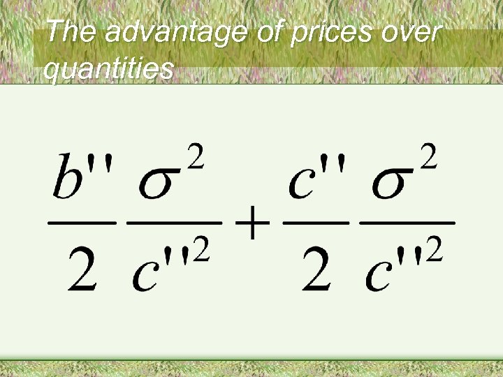
The advantage of prices over quantities
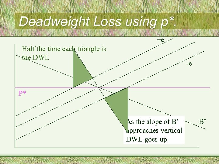
Deadweight Loss using p*. +e Half the time each triangle is the DWL -e P* As the slope of B’ approaches vertical DWL goes up B’
faaead23660867a3780864ee28b7f87a.ppt