PRICE ELASTICITY OF DEMAND When the

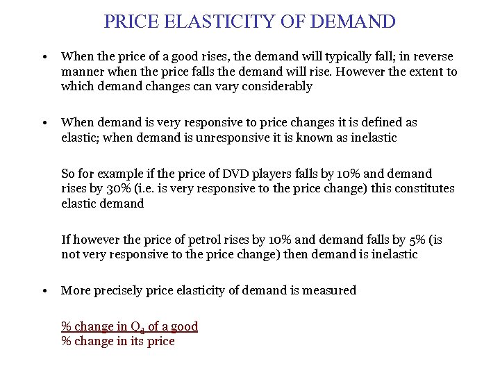PRICE ELASTICITY OF DEMAND • • When the price of a good rises, the demand will typically fall; in reverse manner when the price falls the demand will rise. However the extent to which demand changes can vary considerably When demand is very responsive to price changes it is defined as elastic; when demand is unresponsive it is known as inelastic So for example if the price of DVD players falls by 10% and demand rises by 30% (i. e. is very responsive to the price change) this constitutes elastic demand If however the price of petrol rises by 10% and demand falls by 5% (is not very responsive to the price change) then demand is inelastic • More precisely price elasticity of demand is measured % change in Qd of a good % change in its price

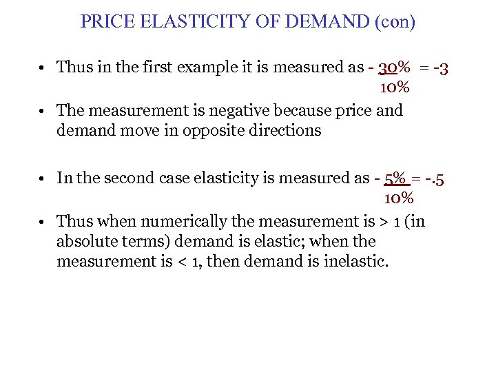PRICE ELASTICITY OF DEMAND (con) • Thus in the first example it is measured as - 30% = -3 10% • The measurement is negative because price and demand move in opposite directions • In the second case elasticity is measured as - 5% = -. 5 10% • Thus when numerically the measurement is > 1 (in absolute terms) demand is elastic; when the measurement is < 1, then demand is inelastic.

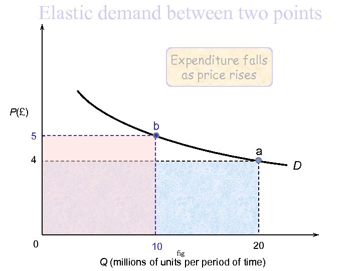Elastic demand between two points Expenditure falls as price rises P(£) 5 b a 4 0 D 10 fig 20 Q (millions of units period of time)

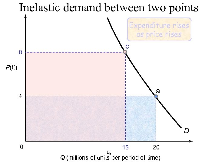Inelastic demand between two points Expenditure rises as price rises c 8 P(£) a 4 D 0 fig 15 20 Q (millions of units period of time)

DETERMINANTS OF PRICE ELASTICITY OF DEMAND Elasticity is determined by a number of factors: • When goods are close substitutes for each other demand tends to be very elastic (>1). By contrast demand is inelastic (< 1) for necessities • Elasticity also depends on the amount of income spent on a good. When a small amount of overall income is spent demand tends to be inelastic • Elasticity also depends on the time period involved. In the short term (e. g. immediately after an alcohol price increase in a budget) demand tends to be very elastic, though much more inelastic in the long run). In other cases demand is more inelastic (e. g. for meat products) in the short than in the long run • Elasticity also depends on whether goods are durable or nondurable

MEASUREMENT OF ELASTICITY • There are two types of measurement of elasticity i. e. arc and point • Though point measurements are more accurate they relate to (theoretical) infinitesmally small changes in price and quantity Arc measurements are used in practice though there is a degree of arbitrariness due to two equally valid ways of calculation (which give opposite answers) So the most correct answer is based on an average of the two other answers Example: If milk is € 1 with 100, 000 bottles sold and then when the price goes up to € 1. 10, 95, 000 bottles are sold. Using old price (P 1) and old quantity (Q 1) as base, PED = - 5, 000/100, 000 divided by 10/100 = -. 5 However using new price (P 2 ) and new quantity (Q 2) as base PED = - 5, 000/95, 000 divided by 10/110 = -. 58 Best measurement = ∆Q/ (Q 1+ Q 2) divided by ∆P/(P 1+ P 2) = -5, 000/195, 000 divided by 10/210 =. 54

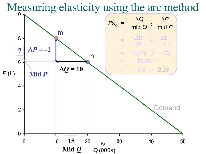Measuring elasticity using the arc method Ped = m = 7 P (£) P = – 2 Mid P Q mid Q 10 15 P ¸ mid P ¸ -2 7 = = = n Q = 10 10/15 x -7/2 -70/30 -7/3 = -2. 33 Demand 15 Mid Q fig Q (000 s)

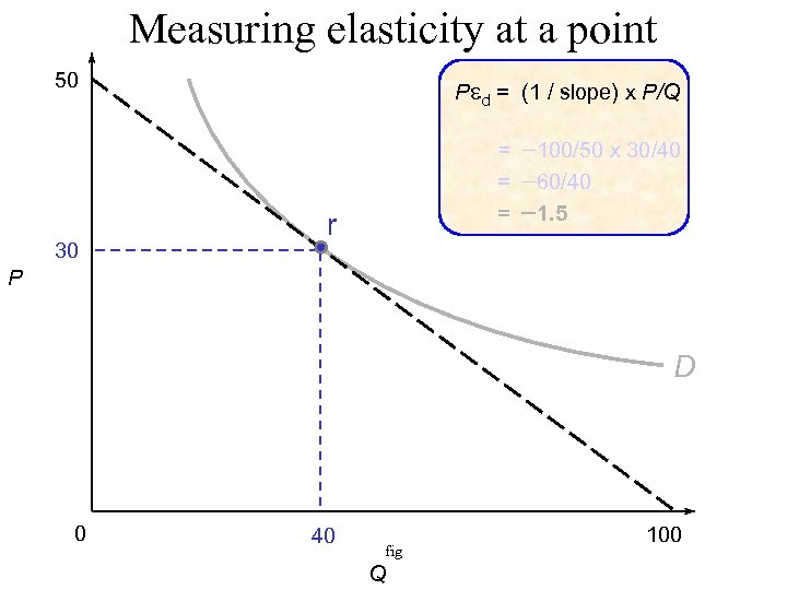Measuring elasticity at a point 50 30 Ped = (1 / slope) x P/Q = = = r -100/50 x 30/40 -60/40 -1. 5 P D 0 40 fig Q 100

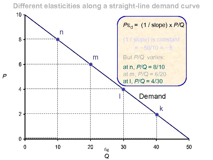Different elasticities along a straight-line demand curve Ped = (1 / slope) x P/Q n (1 / slope) is constant = -50/10 = -5 m But P/Q varies: at n, P/Q = 8/10 at m, P/Q = 6/20 at l, P/Q = 4/30 l P l Demand k fig Q

PRICE ELASTICITY AND CONSUMER EXPENDITURE • The basic rule is as follows If demand is elastic when P increases TR will fall If demand is inelastic when P rises, TR will increase If demand is elastic when P falls, TR will increase If demand is inelastic, when P falls, TR will decrease • In terms of the demand curve elastic demand leads to a more horizontal (flat) shape Inelastic demand leads to a more vertical (steep) curve • If the demand curve is totally horizontal, this represents totally elastic demand (i. e. infinite). If the demand curve is totally vertical, this represents totally inelastic demand (i. e. 0)

IMPORTANT APPLICATIONS OF ELASTICITY • Tax increases with respect to excise duties and VAT by a Government in the budget; for tax revenue to increase demand must be inelastic • Proposed price increases (or decreases) by a company; in the case of monopolies like ESB (where demand for electricity is inelastic) price increases are likely to increase total revenue; in other cases where there are close substitutes such as budget airlines demand is very price elastic so that reductions in fares is more likely to increase revenue • Price elasticity of demand is also very important in both export and import markets For example assuming that export markets such as the UK and US are price competitive (with close substitutes) a rise in the Euro against sterling and the dollar would (other things being equal) lead to a drop in export revenues for Irish firms.

INCOME ELASTICITY OF DEMAND • Income elasticity of demand is also important. It measures the responsiveness of demand to a change in income % change in Qd of a good % change in income • Generally income elasticity is positive. For example an increase in income will lead to increased demand for a product. However for inferior goods demand actually falls as income rises so that income elasticity is negative. • The definition of a normal good is one with a positive income elasticity of demand • Demand is very income elastic for luxuries (e. g. foreign holidays) and income inelastic for necessities (e. g. food). • For a wide range of goods and services income would be the most important determinant of demand; this helps to explain why a recession is so damaging for business

CROSS ELASTICITY OF DEMAND • Cross elasticity of demand measures the responsiveness in demand of one good to a change in price of the other. % change in Qd of good X % change in P of good Y • Cross elasticity is especially important for substitutes and complements. For substitutes (i. e. goods that can be used in place of each other) cross elasticity is measured as positive In other words if the price of Coca Cola was to rise, then the demand for a close substitute (Pepsi Cola) will also rise For complements (i. e. goods that are used jointly) cross elasticity is negative. Thus if the price of petrol was to rise, then the demand for cars will fall (other things remaining equal).

PRICE ELASTICITY OF SUPPLY • • This measures the responsiveness of supply to a change in demand % change in Qs of a good % change in its price If supply changes by more than price (as a %) then supply is elastic. If it changes by less then it is inelastic Supply differs from demand in that it takes a longer time typically for supply to react to price. These time periods are divided into 4 periods as follows Immediate market period, short run, long run, very long run Thus with respect to oil in the immediate market period supply is totally fixed. Therefore any increase in demand will lead to an increase in price. In the short run existing oil wells could be more intensively worked leading to some increase in supply. In the long run new oil wells could be opened up leading to a greater increase in supply. In the very long run the technology of oil production could change leading to further possible increases.

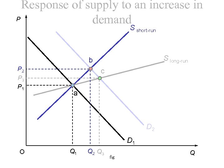Response of supply to an increase in P demand S short-run S long-run b P 2 P 3 P 1 c a D 2 D 1 O Q 1 Q 2 Q 3 fig Q

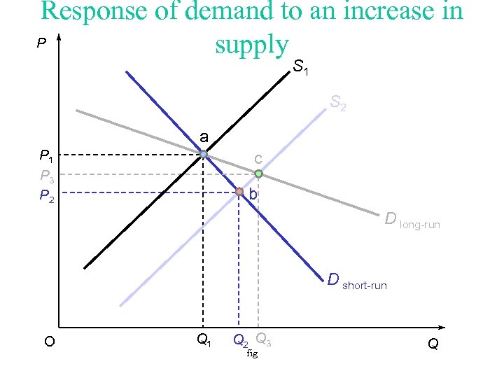Response of demand to an increase in P supply S 1 S 2 a P 1 P 3 P 2 c b D long-run D short-run O Q 1 Q 2 Q 3 fig Q

SPECULATION • Speculation will tend to have a stabilising effect on price fluctuations when suppliers or demanders believe that a change in price is only temporary • Speculation will have a destabilising effect on price fluctuations when suppliers and/or buyers believe that a change in price heralds similar changes to come in the future • Gambling can be of two kinds - when the odds are known (where it is referred to as risk) - when the odds are not known (where it is referred to as uncertainty) The buying of appropriate information can reduce uncertainty Stockholding can also reduce uncertainty

MAXIMUM AND MINIMUM PRICES • Government usually set minimum prices above free market prices (setting a price floor below which prices are not allowed to fall) • Maximum prices are then set below free market prices (setting a price ceiling above which prices are not allowed to rise) • The Common Agricultural Policy is a good example of a minimum price approach • Rent controls provide an interesting example of the alternative maximum price approach

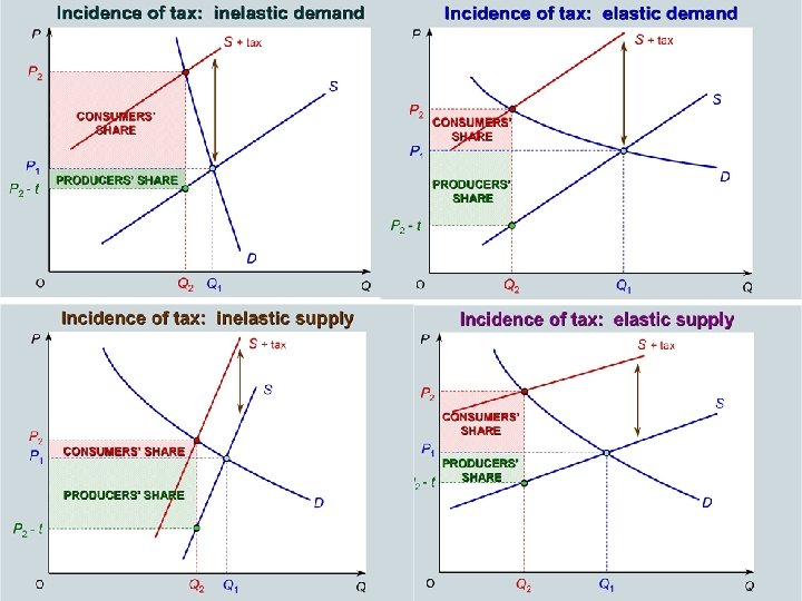
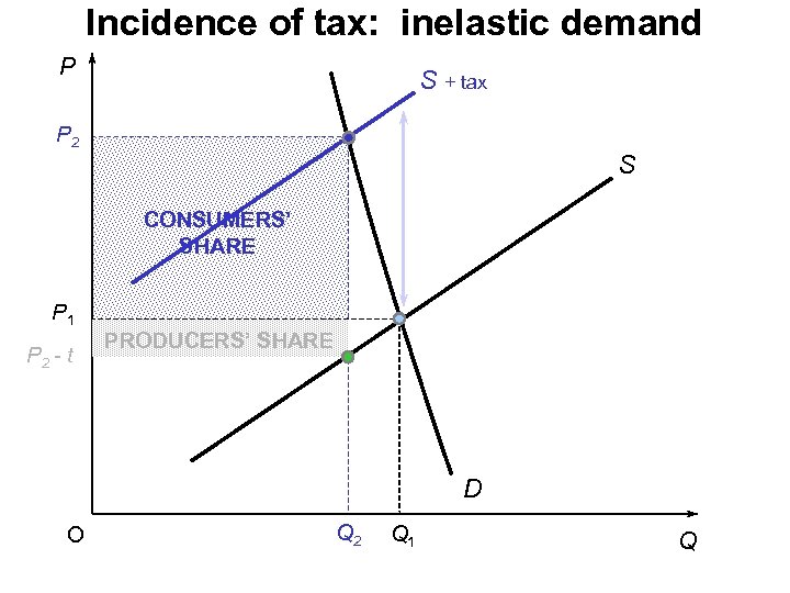Incidence of tax: inelastic demand P S + tax P 2 S CONSUMERS’ SHARE P 1 P 2 - t PRODUCERS’ SHARE D O Q 2 Q 1 Q

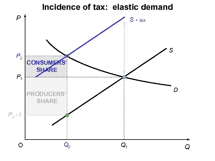Incidence of tax: elastic demand P P 2 S + tax S CONSUMERS’ SHARE P 1 D PRODUCERS’ SHARE P 2 - t O Q 2 Q 1 Q

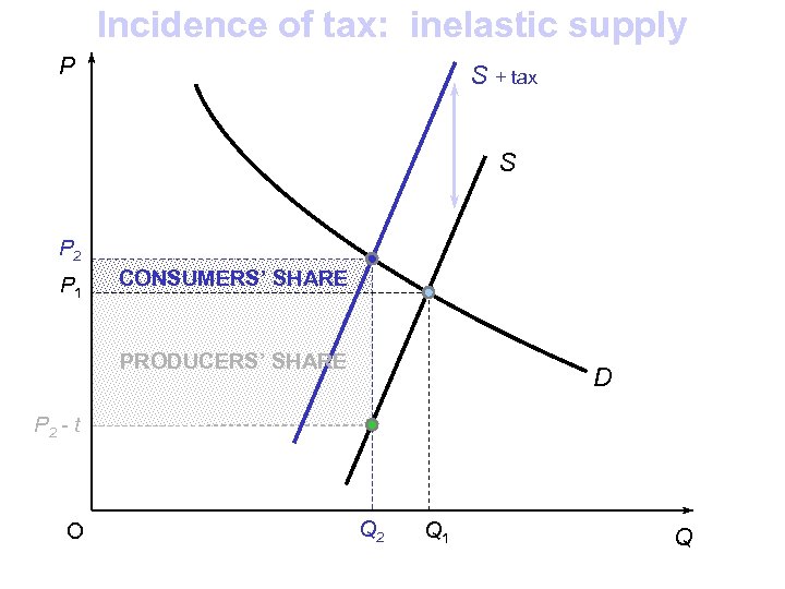Incidence of tax: inelastic supply P S + tax S P 2 P 1 CONSUMERS’ SHARE PRODUCERS’ SHARE D P 2 - t O Q 2 Q 1 Q

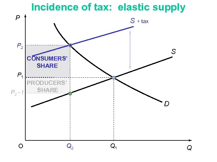Incidence of tax: elastic supply P S + tax P 2 S CONSUMERS’ SHARE P 1 PRODUCERS’ SHARE P 2 - t D O Q 2 Q 1 Q

(UK) Source: National Food Survey 2000 (National Statistics, 2001), extracted from Tables 6. 1, 6. 3, 6. 4 and 6. 5

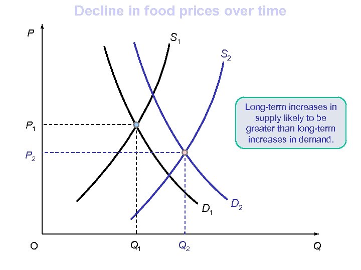Decline in food prices over time P S 1 S 2 Long-term increases in supply likely to be greater than long-term increases in demand. P 1 P 2 D 1 O Q 1 Q 2 D 2 Q

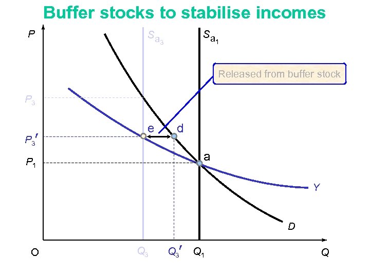Buffer stocks to stabilise incomes P Sa Sa 3 1 Released from buffer stock P 3 ¢ e d a P 1 Y D O Q 3 ¢ Q 1 Q

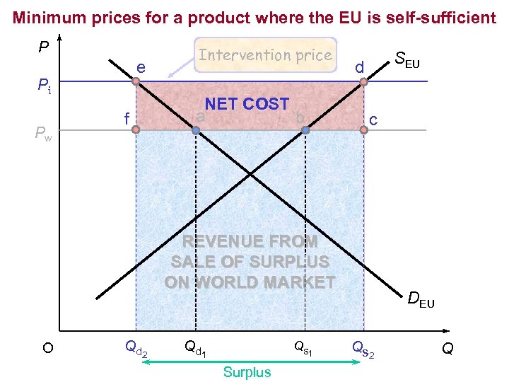Minimum prices for a product where the EU is self-sufficient P e Pi Pw f Intervention price NET COST a b SEU d c COST REVENUE FROM SALE OF SURPLUS ON WORLD MARKET O Q d 2 Qs 1 Q d 1 Surplus DEU Qs 2 Q

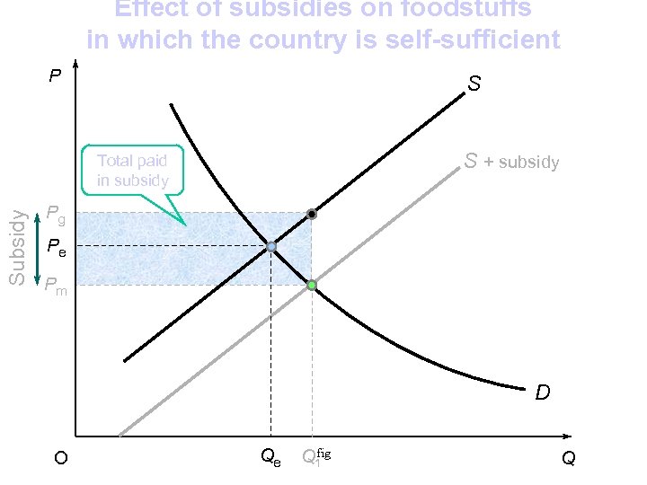Effect of subsidies on foodstuffs in which the country is self-sufficient P S S + subsidy Subsidy Total paid in subsidy Pg Pe Pm D O Qe fig Q 1 Q

MARKET ADJUSTMENT OVER TIME • Full adjustment of price demand supply to a situation of disequilibrium will not be instantaneous • As price elasticities of demand vary with the time period under consideration, the short-term price change can differ from the long-term • If prices are likely to change in the future this will affect the behaviour of buyers and sellers now - a belief that prices will go up (e. g. houses) will cause consumers to buy now; a belief that prices will come down will cause them to postpone present expenditure - a belief that prices will go up will cause producers to postpone selling now; a belief that prices will go down will cause producers to sell now

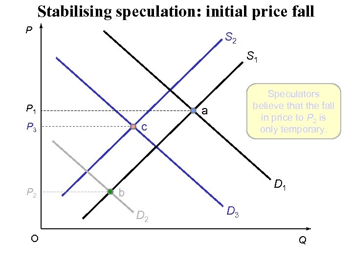Stabilising speculation: initial price fall P S 2 S 1 P 1 a c P 3 P 2 D 1 b D 2 O Speculators believe that the fall in price to P 2 is only temporary. D 3 Q

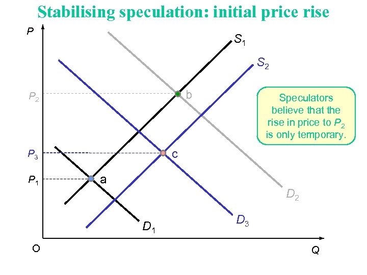Stabilising speculation: initial price rise P S 1 S 2 b P 2 c P 3 P 1 a D 2 D 1 O Speculators believe that the rise in price to P 2 is only temporary. D 3 Q

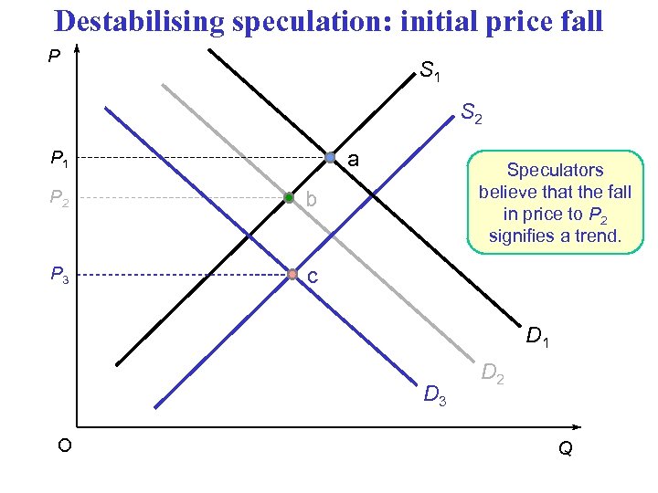Destabilising speculation: initial price fall P S 1 S 2 a P 1 P 2 b P 3 Speculators believe that the fall in price to P 2 signifies a trend. c D 1 D 3 O D 2 Q

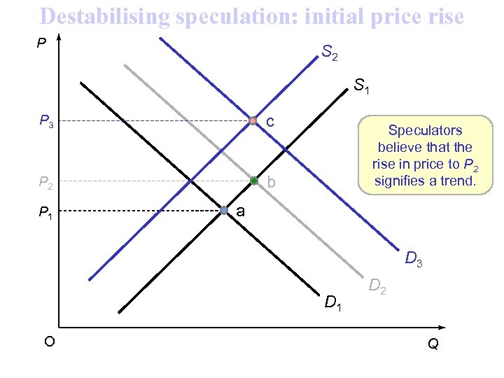Destabilising speculation: initial price rise P S 2 S 1 P 3 c P 2 b P 1 Speculators believe that the rise in price to P 2 signifies a trend. a D 3 D 1 O D 2 Q

MARGINAL UTILITY THEORY • Total and marginal utility • meaning of total utility – marginal utility: TU/ Q • diminishing marginal utility: as the consumption of a product increases (assuming no significant time delay as between units) the extra utility or satisfaction experienced on each additional unit consumed tends to diminish and in extremes become negative - marginal utility: TU/ Q for example if one consumes four cups of coffee in one session, the utility of the marginal unit (i. e. each additional cup of coffee) will diminish - total and marginal utility curves

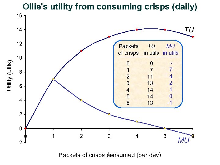Ollie's utility from consuming crisps (daily) TU Utility (utils) MU Packets TU of crisps in utils 0 1 2 3 4 5 6 0 7 11 13 14 14 13 7 4 2 1 0 -1 MU fig Packets of crisps consumed (per day)

MARGINAL UTILITY THEORY • The optimum level of consumption: the one-commodity version – consumer surplus is the notion that a consumer can gain a surplus of utility. For example using a previous example if one is willing to pay € 2 for the each of the four cups of coffee consumed then this implies that the utility from the last cup justifies the price paid. Therefore as the marginal utility is higher on the 1 st, 2 nd and 3 rd units, then one thereby obtains surplus utility on the earlier units consumed • marginal consumer surplus: MU – P • total consumer surplus: TU – TE • maximising consumer surplus: P = MU • Marginal utility and the demand curve

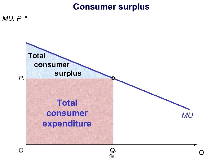Consumer surplus MU, P P 1 Total consumer surplus Total consumer expenditure O MU Q 1 fig Q