Price Discrimination 1 Introduction Price Discrimination

Price Discrimination 1

Introduction • Price Discrimination describes strategies used by firms to extract surplus from customers 2

Mechanisms for Capturing Surplus • Market segmentation • Non-linear pricing – Two-part pricing – Block pricing • Tying and bundling • Quality discrimination 3

Feasibility of price discrimination • Market power • Two problems confront a firm wishing to price discriminate – identification: the firm is able to identify demands of different types of consumer or in separate markets – arbitrage: prevent consumers who are charged a low price from reselling to consumers who are charged a high price • The firm then must choose the type of price discrimination – first-degree or personalized pricing – second-degree or menu pricing – third-degree or group pricing 4

Third-degree price discrimination • Consumers differ by some observable characteristic(s) • A uniform price is charged to all consumers in a particular group – linear price • Different uniform prices are charged to different groups – “kids are free” – subscriptions to professional journals e. g. American Economic Review – Airlines – early-bird specials 5

Third-degree price discrimination 2 • The pricing rule is very simple: – consumers with low elasticity of demand should be charged a high price – consumers with high elasticity of demand should be charged a low price 6

Third degree price discrimination: example • Harry Potter volume sold in the United States and Europe • Demand: – United States: PU = 36 – 4 QU – Europe: PE = 24 – 4 QE • Marginal cost constant in each market – MC = $4 7

The example: no price discrimination • Suppose that the same price is charged in both markets • Use the following procedure: – calculate aggregate demand in the two markets – identify marginal revenue for that aggregate demand – equate marginal revenue with marginal cost to identify the profit maximizing quantity – identify the market clearing price from the aggregate demand – calculate demands in the individual markets from the individual market demand curves and the equilibrium price 8

The example (cont. ) United States: PU = 36 – 4 QU Invert this: QU = 9 – P/4 for P < $36 Europe: PU = 24 – 4 QE Invert QE = 6 – P/4 for P < $24 Aggregate these demands Q = QU + QE = 9 – P/4 for $36 ≥ P ≥ Q = QU + QE = 15 – P/2 for P < $24 At these prices only the US market is active Now both markets are $24 active 9

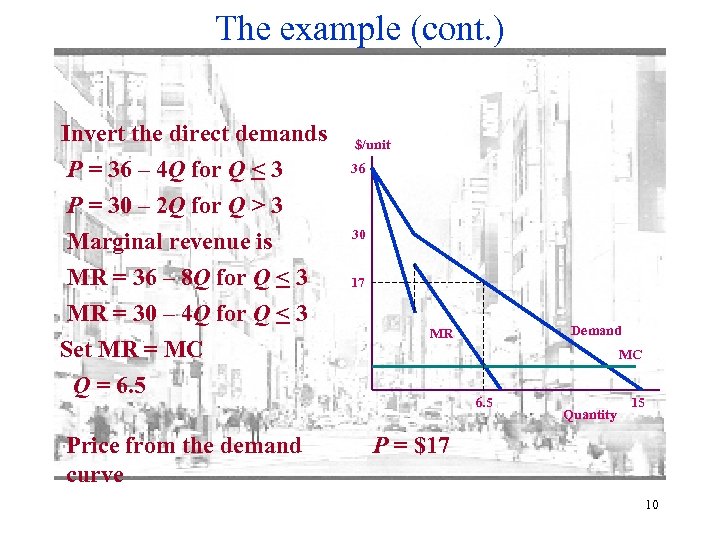The example (cont. ) Invert the direct demands P = 36 – 4 Q for Q < 3 P = 30 – 2 Q for Q > 3 Marginal revenue is MR = 36 – 8 Q for Q < 3 MR = 30 – 4 Q for Q < 3 Set MR = MC Q = 6. 5 Price from the demand curve $/unit 36 30 17 Demand MR MC 6. 5 Quantity 15 P = $17 10

The example (cont. ) Substitute price into the individual market demand curves: QU = 9 – P/4 = 9 – 17/4 = 4. 75 million QE = 6 – P/4 = 6 – 17/4 = 1. 75 million Aggregate profit = (17 – 4)x 6. 5 = $84. 5 million 11

The example: price discrimination • The firm can improve on this outcome • Check that MR is not equal to MC in both markets – MR > MC in Europe – MR < MC in the US – the firms should transfer some books from the US to Europe • This requires that different prices be charged in the two markets • Procedure: – take each market separately – identify equilibrium quantity in each market by equating MR and MC – identify the price in each market from market demand 12

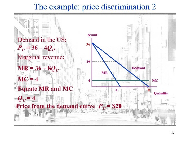The example: price discrimination 2 Demand in the US: PU = 36 – 4 QU Marginal revenue: MR = 36 – 8 QU $/unit 36 20 Demand MR MC = 4 4 Equate MR and MC 4 QU = 4 Price from the demand curve PU = $20 MC 9 Quantity 13

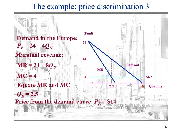The example: price discrimination 3 Demand in the Europe: PE = 24 – 4 QU Marginal revenue: MR = 24 – 8 QU $/unit 24 14 Demand MR MC = 4 4 Equate MR and MC 2. 5 QE = 2. 5 Price from the demand curve PE = $14 MC 6 Quantity 14

The example: price discrimination 4 • Aggregate sales are 6. 5 million books – the same as without price discrimination • Aggregate profit is (20 – 4)x 4 + (14 – 4)x 2. 5 = $89 million – $4. 5 million greater than without price discrimination 15

No price discrimination: non-constant cost • The example assumes constant marginal cost • How is this affected if MC is non-constant? – Suppose MC is increasing • No price discrimination procedure – – – Calculate aggregate demand Calculate the associated MR Equate MR with MC to give aggregate output Identify price from aggregate demand Identify market demands from individual demand curves 16

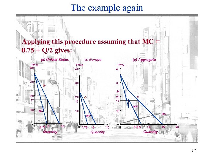The example again Applying this procedure assuming that MC = 0. 75 + Q/2 gives: (a) United States Price 40 (c) Aggregate (b) Europe Price 40 30 30 DU Price 40 30 24 20 17 DE D MR 10 U MR 10 10 MC E MR 0 0 4. 75 5 Quantity 10 0 0 1. 75 5 Quantity 10 0 0 5 6. 5 10 15 20 Quantity 17

Price discrimination: non-constant cost • With price discrimination the procedure is – Identify marginal revenue in each market – Aggregate these marginal revenues to give aggregate marginal revenue – Equate this MR with MC to give aggregate output – Identify equilibrium MR from the aggregate MR curve – Equate this MR with MC in each market to give individual market quantities – Identify equilibrium prices from individual market demands 18

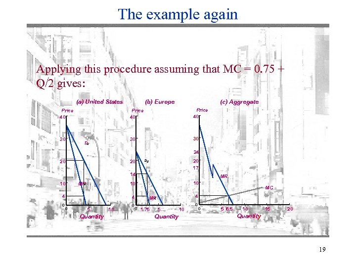The example again Applying this procedure assuming that MC = 0. 75 + Q/2 gives: (a) United States Price 40 DU Price 40 30 (c) Aggregate (b) Europe 30 24 20 20 20 17 DE 14 10 4 0 MR 10 10 U MR 5 Quantity 10 0 4 E MR 0 1. 75 MC 5 Quantity 10 0 0 5 6. 5 10 15 20 Quantity 19

Some additional comments • Suppose that demands are linear – price discrimination results in the same aggregate output as no price discrimination – price discrimination increases profit • For any demand specifications two rules apply – marginal revenue must be equalized in each market – marginal revenue must equal aggregate marginal cost 20

Third-degree price discrimination 2 • Often arises when firms sell differentiated products – hard-back versus paper back books – first-class versus economy airfare • Price discrimination exists in these cases when: – “two varieties of a commodity are sold by the same seller to two buyers at different net prices, the net price being the price paid by the buyer corrected for the cost associated with the product differentiation. ” (Phlips) • The seller needs an easily observable characteristic that signals willingness to pay • The seller must be able to prevent arbitrage – e. g. require a Saturday night stay for a cheap flight 21

Other mechanisms for price discrimination • Impose restrictions on use to control arbitrage – – Saturday night stay no changes/alterations personal use only (academic journals) time of purchase (movies, restaurants) • Damaged goods • Discrimination by location 22

Discrimination by location • Suppose demand in two distinct markets is identical – Pi = A = BQi • But suppose that there are different marginal costs in supplying the two markets – cj = ci + t • Profit maximizing rule: – – equate MR with MC in each market as before Pi = (A + ci)/2; Pj = (A + ci + t)/2 Pj – Pi = t/2 cj – ci difference in prices is not the same as the difference in costs 23

Introduction to Nonlinear Pricing • Annual subscriptions generally cost less in total than one-off purchases • Buying in bulk usually offers a price discount – these are price discrimination reflecting quantity discounts – prices are nonlinear, with the unit price dependent upon the quantity bought – allows pricing nearer to willingness to pay – so should be more profitable than third-degree price discrimination • How to design such pricing schemes? – depends upon the information available to the seller about buyers – distinguish first-degree (personalized) and second-degree (menu) pricing 24

First-degree price discrimination 2 • Monopolist can charge maximum price that each consumer is willing to pay • Extracts all consumer surplus • Since profit is now total surplus, find that first-degree price discrimination is efficient 25

First-degree price discrimination 3 • First-degree price discrimination is highly profitable but requires – detailed information – ability to avoid arbitrage • Leads to the efficient choice of output: since price equals marginal revenue and MR = MC – no value-creating exchanges are missed 26

First-degree price discrimination 4 • The information requirements appear to be insurmountable – but not in particular cases • tax accountants, doctors, students applying to private universities • But there are pricing schemes that will achieve the same outcome – non-linear prices – two-part pricing as a particular example of non-linear prices • charge a quantity-independent fee (membership? ) plus a per unit usage charge – block pricing is another • bundle total charge and quantity in a package 27

Two-part pricing • Jazz club serves two types of customer – Old: demand for entry plus Qo drinks is P = Vo – Qo – Young: demand for entry plus Qy drinks is P = Vy – Qy – Equal numbers of each type – Assume that Vo > Vy: Old are willing to pay more than Young – Cost of operating the jazz club C(Q) = F + c. Q • Demand costs are all in daily units 28

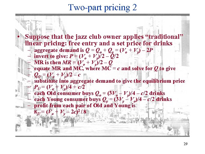Two-part pricing 2 • Suppose that the jazz club owner applies “traditional” linear pricing: free entry and a set price for drinks – – – – – aggregate demand is Q = Qo + Qy = (Vo + Vy) – 2 P invert to give: P = (Vo + Vy)/2 – Q/2 MR is then MR = (Vo + Vy)/2 – Q equate MR and MC, where MC = c and solve for Q to give QU = (Vo + Vy)/2 – c substitute into aggregate demand to give the equilibrium price PU = (Vo + Vy)/4 + c/2 each Old consumer buys Qo = (3 Vo – Vy)/4 – c/2 drinks each Young consumer buys Qy = (3 Vy – Vo)/4 – c/2 drinks profit from each pair of Old and Young is U = (Vo + Vy – 2 c)2 / 8 29

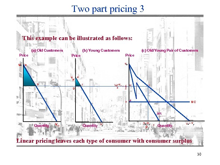Two part pricing 3 This example can be illustrated as follows: (a) Old Customers Price Vo (b) Young Customers Price Vo a V d (c) Old/Young Pair of Customers y b e f Vo+V y + c h 4 2 i c k g j MC MR Quantity Vo Quantity Vy Vo+V y 2 -c Quantity Vo + Vy Linear pricing leaves each type of consumer with consumer surplus 30

Two part pricing 4 • Jazz club owner can do better than this • Consumer surplus at the uniform linear price is: – Old: CSo = (Vo – PU). Qo/2 = (Qo)2/2 – Young: CSy = (Vy – PU). Qy/2 = (Qy)2/2 • So charge an entry fee (just less than): – Eo = CSo to each Old customer and Ey = CSy to each Young customer • check IDs to implement this policy – each type will still be willing to frequent the club and buy the equilibrium number of drinks • So this increases profit by Eo for each Old and Ey for each Young customer 31

Two part pricing 5 • The jazz club can do even better – reduce the price per drink – this increases consumer surplus – but the additional consumer surplus can be extracted through a higher entry fee • Consider the best that the jazz club owner can do with respect to each type of consumer 32

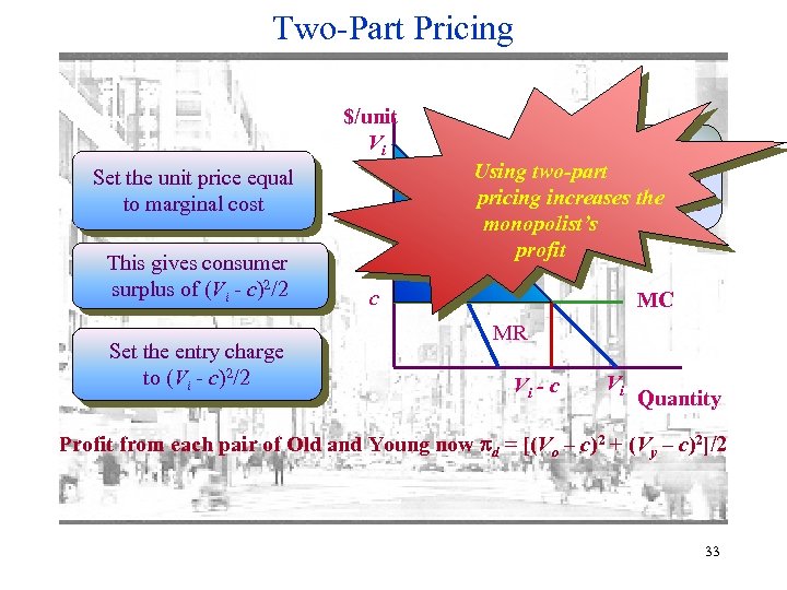Two-Part Pricing $/unit Vi Set the unit price equal to marginal cost This gives consumer surplus of (Vi - c)2/2 Set the entry charge to (Vi - c)2/2 The entry charge Using two-part consumer converts pricing surplus into profit increases the monopolist’s profit c MC MR Vi - c Vi Quantity Profit from each pair of Old and Young now d = [(Vo – c)2 + (Vy – c)2]/2 33

Block pricing • There is another pricing method that the club owner can apply – offer a package of “Entry plus X drinks for $Y” • To maximize profit apply two rules – set the quantity offered to each consumer type equal to the amount that type would buy at price equal to marginal cost – set the total charge for each consumer type to the total willingness to pay for the relevant quantity • Return to the example: 34

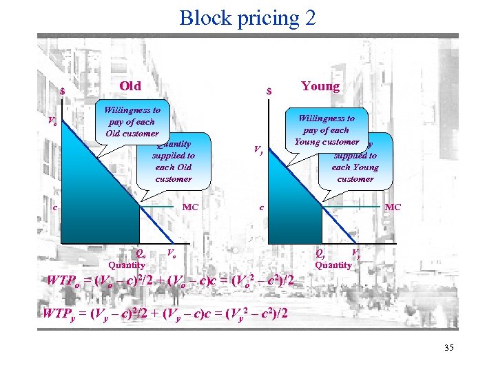Block pricing 2 $ Vo Old $ Willingness to pay of each Old customer Quantity supplied to each Old customer c MC Qo Quantity Vy Young Willingness to pay of each Young customer Quantity supplied to each Young customer c Vo MC Qy Vy Quantity WTPo = (Vo – c)2/2 + (Vo – c)c = (Vo 2 – c 2)/2 WTPy = (Vy – c)2/2 + (Vy – c)c = (Vy 2 – c 2)/2 35

Block pricing 3 • How to implement this policy? 36

Second-degree price discrimination • What if the seller cannot distinguish between buyers? – perhaps they differ in income (unobservable) • Then the type of price discrimination just discussed is impossible • High-income buyer will pretend to be a low-income buyer – to avoid the high entry price – to pay the smaller total charge • Take a specific example – Ph = 16 – Qh – Pl = 12 – Ql – MC = 4 37

Second-degree price discrimination 2 • First-degree price discrimination requires: – High Income: entry fee $72 and $4 per drink or entry plus 12 drinks for a total charge of $120 – Low Income: entry fee $32 and $4 per drink or entry plus 8 drinks for total charge of $64 • This will not work – high income types get no consumer surplus from the package designed for them but get consumer surplus from the other package – so they will pretend to be low income even if this limits the number of drinks they can buy • Need to design a “menu” of offerings targeted at the two types 38

Second-degree price discrimination 3 • The seller has to compromise • Design a pricing scheme that makes buyers – reveal their true types – self-select the quantity/price package designed for them • Essence of second-degree price discrimination • It is “like” first-degree price discrimination – the seller knows that there are buyers of different types – but the seller is not able to identify the different types • A two-part tariff is ineffective • Use quantity discounting 39

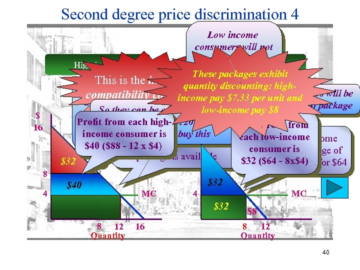Second degree price discrimination 4 Low income consumers will not buy the ($88, 12) High-income Low-Income package since exhibit These packagesthey This is the incentive are willing to pay highquantity discounting: So any So will the high- other package for 12 consumers will be compatibility constraint only $72 per unit and income. The low-demand pay $7. 33 income consumers: high-income to buy this ($64, 8) package offered to willing drinks low-income pay $8 So they can be 8) offered a package because consumers must offer at the ($64, $ High high. Profit from each(since $120 - 32 = are And profit from of ($88, 12)income consumers 88) package gives them $32 willing to pay least $32 will up to $120 for each low-income consumer surplus Offer the low-income and they consumer surplusis buy this 12 entry x $4) $40 ($88 - 12 plus 12 drinks if no other consumers a package of consumer is package is available $32 ($64 - 8 drinks for $64 $32 entry plus 8 x$4) $ 16 8 4 $32 $40 $64 $32 $8 $24 $32 MC $16 8 12 Quantity 4 MC $32 16 $8 8 12 Quantity 40

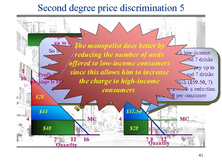Second degree price discrimination 5 A high-income consumer will pay High-Income up to $87. 50 for entry and 7 The monopolist does better by So buying thedrinks 7) package ($59. 50, Suppose reducing the number of units each low-income gives him $28 consumer surplus consumer is offered 7 drinks offered to can beclub. Can the sold So entry plus 12 drinks low-income consumers Each consumer will pay up to Low-Income for entry and 7 drinks for $92 ($92, 28 = $92) $ since owner do even this $59. 50 Profit from each($120 -12) allows him to increase $ 16 package is $44: an increase of $4 to this? the charge high-income from eachnumber 7) Yes! Reduce the ($59. 50, Profit better than 12 per consumer package is $31. 50: reduction of units offered toaeach consumers of $0. 50 consumer low-incomeper consumer $28 4 $87. 50 $44$92 MC $28 $48 4 $31. 50 $59. 50 MC $28 7 12 Quantity 16 7 8 12 Quantity 41

Second-degree price discrimination 6 • Will the monopolist always want to supply both types of consumer? • There are cases where it is better to supply only highdemand types – high-class restaurants – golf and country clubs • Take our example again – suppose that there are Nl low-income consumers – and Nh high-income consumers 42

Second-degree price discrimination 7 • Suppose both types of consumer are served – two packages are offered ($57. 50, 7) aimed at low-income and ($92, 12) aimed at high-income – profit is $31. 50 x. Nl + $44 x. Nh • Now suppose only high-income consumers are served – then a ($120, 12) package can be offered – profit is $72 x. Nh • Is it profitable to serve both types? – Only if $31. 50 x. Nl + $44 x. Nh > $72 x. Nh 31. 50 Nl > 28 Nh This requires that Nh < 31. 50 = 1. 125 Nl 28 There should not be “too high” a fraction of high-demand consumers 43

Second-degree price discrimination 8 • Characteristics of second-degree price discrimination – extract all consumer surplus from the lowest-demand group – leave some consumer surplus for other groups – offer less than the socially efficient quantity to all groups other than the highest-demand group – offer quantity-discounting • Second-degree price discrimination converts consumer surplus into profit less effectively than first-degree • Some consumer surplus is left “on the table” in order to induce high-demand groups to buy large quantities 44

Tying • Tying is a seller’s conditioning the purchase of one product on the purchase of another – Technological ties • Printer cartridges – Contractual ties • Car dealer and car parts • Why tying? 45

Quality Discrimination • Why is Quality Discrimination a form of Price Discrimination? – First / business class airfare vs economy class • Reduction in quality of the lower-quality good to reduce the incentive of people with high willingness to pay to switch from the high-quality good when the firm increases its price – “Damaged goods” 46