Презентация Week 10 Aggregate Demand and Aggregate Supply

10 AGGREGATE SUPPLY AND AGGREGATE DEMAN

© 2012 Pearson Addison-Wesley

© 2012 Pearson Addison-Wesley Production grows and prices rise, but the pace is uneven. In 2004, U. S. real GDP grew by 3. 6 percent. In 2008, U. S. real GDP had zero growth. In 2009, U. S. real GDP shrank by more than 2 percent. During these years, prices increased by between 3 percent (in 2005) and 1 percent (in 2009). What forces bring an uneven expansion of real GDP? What forces cause the business cycle? How are real GDP and the price level determined?

© 2012 Pearson Addison-Wesley Quantity Supplied and Supply The quantity of real GDP supplied is the total quantity that firms plan to produce during a given period. Aggregate supply is the relationship between the quantity of real GDP supplied and the price level. We distinguish two time frames associated with different states of the labor market: Long-run aggregate supply Short-run aggregate supply Aggregate Supply

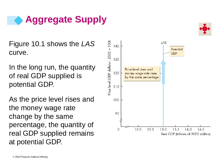
© 2012 Pearson Addison-Wesley Long-Run Aggregate Supply Long-run aggregate supply is the relationship between the quantity of real GDP supplied and the price level when real GDP equals potential GDP. Potential GDP is independent of the price level. So the long-run aggregate supply curve ( LAS ) is vertical at potential GDP. Aggregate Supply

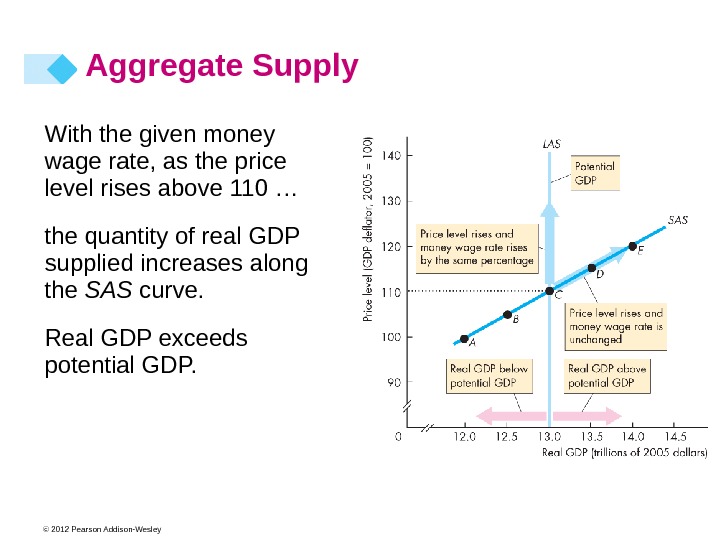
© 2012 Pearson Addison-Wesley. Short-Run Aggregate Supply Short-run aggregate supply is the relationship between the quantity of real GDP supplied and the price level when the money wage rate, the prices of other resources, and potential GDP remain constant. A rise in the price level with no change in the money wage rate and other factor prices increases the quantity of real GDP supplied. The short-run aggregate supply curve ( SAS ) is upward sloping. Aggregate Supply

© 2012 Pearson Addison-Wesley. Figure 10. 1 shows the LAS curve. In the long run, the quantity of real GDP supplied is potential GDP. As the price level rises and the money wage rate change by the same percentage, the quantity of real GDP supplied remains at potential GDP. Aggregate Supply

© 2012 Pearson Addison-Wesley In the short run, the quantity of real GDP supplied increases if the price level rises. The SAS curve slopes upward. A rise in the price level with no change in the money wage rate induces firms to increase production. Aggregate Supply

© 2012 Pearson Addison-Wesley With a given money wage rate, the SAS curve cuts the LAS curve at potential GDP. The price level is 110. With the given money wage rate, as the price level falls below 110. . . the quantity of real GDP supplied decreases along the SAS curve. Aggregate Supply

© 2012 Pearson Addison-Wesley With the given money wage rate, as the price level rises above 110 … the quantity of real GDP supplied increases along the SAS curve. Real GDP exceeds potential GDP. Aggregate Supply

© 2012 Pearson Addison-Wesley. Changes in Aggregate Supply Aggregate supply changes if an influence on production plans other than the price level changes. These influences include Changes in potential GDP Changes in money wage rate (and other factor prices) Aggregate Supply

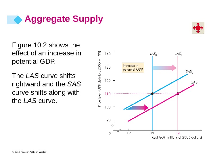
© 2012 Pearson Addison-Wesley Changes in Potential GDP When potential GDP increases, both the LAS and SAS curves shift rightward. Potential GDP changes, for three reasons: An increase in the full-employment quantity of labor changes An increase in the quantity of capital (physical or human) changes An advance in technology Aggregate Supply

© 2012 Pearson Addison-Wesley. Figure 10. 2 shows the effect of an increase in potential GDP. The LAS curve shifts rightward and the SAS curve shifts along with the LAS curve. Aggregate Supply

© 2012 Pearson Addison-Wesley. Changes in the Money Wage Rate Figure 10. 3 shows the effect of a rise in the money wage rate. Short-run aggregate supply decreases and the SAS curve shifts leftward. Long-run aggregate supply does not change. Aggregate Supply

© 2012 Pearson Addison-Wesley The quantity of real GDP demanded, Y , is the total amount of final goods and services produced in the United States that people, businesses, governments, and foreigners plan to buy. This quantity is the sum of consumption expenditures, C , investment, I , government expenditure, G , and net exports, X – M. That is, Y = C + I + G + X – M. Aggregate Demand

© 2012 Pearson Addison-Wesley Buying plans depend on many factors and some of the main ones are The price level Expectations Fiscal policy and monetary policy The world economy Aggregate Demand

© 2012 Pearson Addison-Wesley Aggregate Demand The Aggregate Demand Curve Aggregate demand is the relationship between the quantity of real GDP demanded and the price level. The aggregate demand curve ( AD ) plots the quantity of real GDP demanded against the price level.

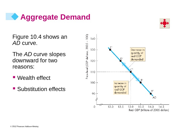
© 2012 Pearson Addison-Wesley Figure 10. 4 shows an AD curve. The AD curve slopes downward for two reasons: Wealth effect Substitution effects Aggregate Demand

© 2012 Pearson Addison-Wesley Aggregate Demand Wealth Effect A rise in the price level, other things remaining the same, decreases the quantity of real wealth (money, stocks, etc. ). To restore their real wealth, people increase saving and decrease spending. The quantity of real GDP demanded decreases. Similarly, a fall in the price level, other things remaining the same, increases the quantity of real wealth and increases the quantity of real GDP demanded increases.

© 2012 Pearson Addison-Wesley Aggregate Demand Substitution Effects Intertemporal substitution effect : A rise in the price level, other things remaining the same, decreases the real value of money and raises the interest rate. When the interest rate rises, people borrow and spend less, so the quantity of real GDP demanded decreases. Similarly, a fall in the price level increases the real value of money and lowers the interest rate. When the interest rate falls, people borrow and spend more, so the quantity of real GDP demanded increases.

© 2012 Pearson Addison-Wesley Aggregate Demand International substitution effect : A rise in the price level, other things remaining the same, increases the price of domestic goods relative to foreign goods. So imports increase and exports decrease, which decreases the quantity of real GDP demanded. Similarly, a fall in the price level, other things remaining the same, increases the quantity of real GDP demanded.

© 2012 Pearson Addison-Wesley Aggregate Demand Changes in Aggregate Demand A change in any influence on buying plans other than the price level changes aggregate demand. The main influences on aggregate demand are Expectations Fiscal policy and monetary policy The world economy

© 2012 Pearson Addison-Wesley Aggregate Demand Expectations about future income, future inflation, and future profits change aggregate demand. Increases in expected future income increase people’s consumption today and increases aggregate demand. A rise in the expected inflation rate makes buying goods cheaper today and increases aggregate demand. An increase in expected future profits boosts firms’ investment, which increases aggregate demand.

© 2012 Pearson Addison-Wesley Aggregate Demand Fiscal Policy and Monetary Policy Fiscal policy is the government’s attempt to influence the economy by setting and changing taxes, making transfer payments, and purchasing goods and services. A tax cut or an increase in transfer payments increases households’ disposable income —aggregate income minus taxes plus transfer payments. An increase in disposable income increases consumption expenditure and increases aggregate demand.

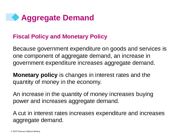
© 2012 Pearson Addison-Wesley Aggregate Demand Fiscal Policy and Monetary Policy Because government expenditure on goods and services is one component of aggregate demand, an increase in government expenditure increases aggregate demand. Monetary policy is changes in interest rates and the quantity of money in the economy. An increase in the quantity of money increases buying power and increases aggregate demand. A cut in interest rates increases expenditure and increases aggregate demand.

© 2012 Pearson Addison-Wesley Aggregate Demand The World Economy The world economy influences aggregate demand in two ways: A fall in the foreign exchange rate lowers the price of domestic goods and services relative to foreign goods and services, which increases exports, decreases imports, and increases aggregate demand. An increase in foreign income increases the demand for U. S. exports and increases aggregate demand.

© 2012 Pearson Addison-Wesley Aggregate Demand Figure 10. 5 illustrates changes in aggregate demand. When aggregate demand increases, the AD curve shifts rightward… … and when aggregate demand decreases, the AD curve shifts leftward.

© 2012 Pearson Addison-Wesley Explaining Macroeconomic Trends and Fluctuations Short-Run Macroeconomic Equilibrium Short-run macroeconomic equilibrium occurs when the quantity of real GDP demanded equals the quantity of real GDP supplied at the point of intersection of the AD curve and the SAS curve.

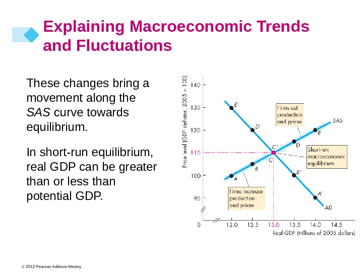
© 2012 Pearson Addison-Wesley Figure 10. 6 illustrates a short-run equilibrium. If real GDP is below equilibrium GDP, firms increase production and raise prices… … and if real GDP is above equilibrium GDP, firms decrease production and lower prices. Explaining Macroeconomic Trends and Fluctuations

© 2012 Pearson Addison-Wesley These changes bring a movement along the SAS curve towards equilibrium. In short-run equilibrium, real GDP can be greater than or less than potential GDP. Explaining Macroeconomic Trends and Fluctuations

© 2012 Pearson Addison-Wesley Long-Run Macroeconomic Equilibrium Long-run macroeconomic equilibrium occurs when real GDP equals potential GDP—when the economy is on its LAS curve. Long-run equilibrium occurs at the intersection of the AD and LAS curves. Explaining Macroeconomic Trends and Fluctuations

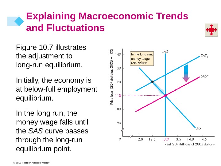
© 2012 Pearson Addison-Wesley Figure 10. 7 illustrates the adjustment to long-run equilibrium. Initially, the economy is at below-full employment equilibrium. In the long run, the money wage falls until the SAS curve passes through the long-run equilibrium point. Explaining Macroeconomic Trends and Fluctuations

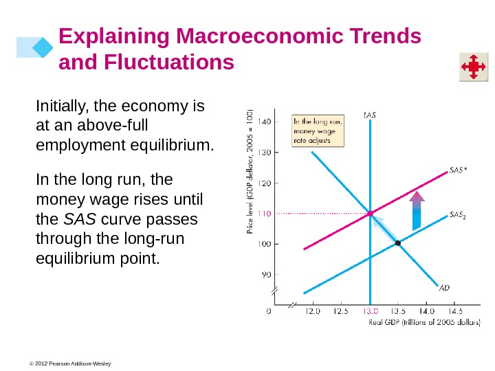
© 2012 Pearson Addison-Wesley Initially, the economy is at an above-full employment equilibrium. In the long run, the money wage rises until the SAS curve passes through the long-run equilibrium point. Explaining Macroeconomic Trends and Fluctuations

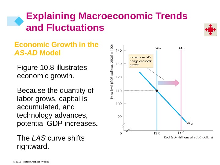
© 2012 Pearson Addison-Wesley Economic Growth in the AS — AD Model Figure 10. 8 illustrates economic growth. Because the quantity of labor grows, capital is accumulated, and technology advances, potential GDP increases. The LAS curve shifts rightward. Explaining Macroeconomic Trends and Fluctuations

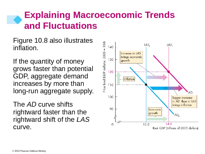
© 2012 Pearson Addison-Wesley Figure 10. 8 also illustrates inflation. If the quantity of money grows faster than potential GDP, aggregate demand increases by more than long-run aggregate supply. The AD curve shifts rightward faster than the rightward shift of the LAS curve. Explaining Macroeconomic Trends and Fluctuations

© 2012 Pearson Addison-Wesley The Business Cycle in the AS — AD Model The business cycle occurs because aggregate demand the short-run aggregate supply fluctuate, but the money wage does not change rapidly enough to keep real GDP at potential GDP. An above full-employment equilibrium is an equilibrium in which real GDP exceeds potential GDP. A full-employment equilibrium is an equilibrium in which real GDP equals potential GDP. A below full-employment equilibrium is an equilibrium in which potential GDP exceeds real GDP. Explaining Macroeconomic Trends and Fluctuations

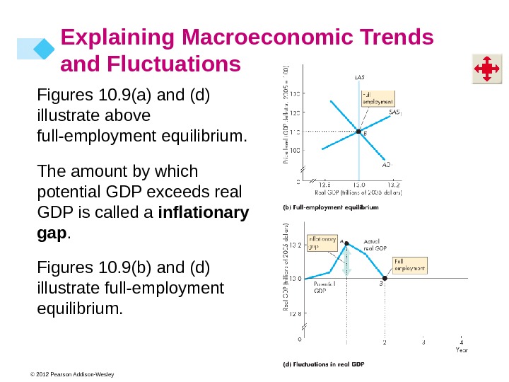
© 2012 Pearson Addison-Wesley Figures 10. 9(a) and (d) illustrate above full-employment equilibrium. The amount by which potential GDP exceeds real GDP is called a inflationary gap. Figures 10. 9(b) and (d) illustrate full-employment equilibrium. Explaining Macroeconomic Trends and Fluctuations

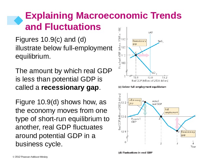
© 2012 Pearson Addison-Wesley Figures 10. 9(c) and (d) illustrate below full-employment equilibrium. The amount by which real GDP is less than potential GDP is called a recessionary gap. Figure 10. 9(d) shows how, as the economy moves from one type of short-run equilibrium to another, real GDP fluctuates around potential GDP in a business cycle. Explaining Macroeconomic Trends and Fluctuations

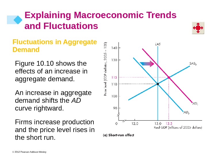
© 2012 Pearson Addison-Wesley Fluctuations in Aggregate Demand Figure 10. 10 shows the effects of an increase in aggregate demand. An increase in aggregate demand shifts the AD curve rightward. Firms increase production and the price level rises in the short run. Explaining Macroeconomic Trends and Fluctuations

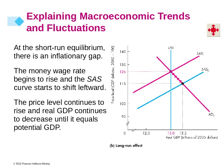
© 2012 Pearson Addison-Wesley At the short-run equilibrium, there is an inflationary gap. The money wage rate begins to rise and the SAS curve starts to shift leftward. The price level continues to rise and real GDP continues to decrease until it equals potential GDP. Explaining Macroeconomic Trends and Fluctuations

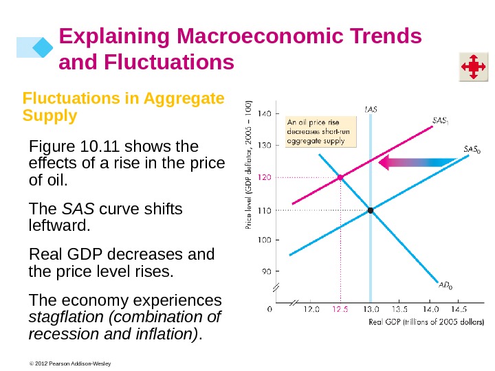
© 2012 Pearson Addison-Wesley. Fluctuations in Aggregate Supply Figure 10. 11 shows the effects of a rise in the price of oil. The SAS curve shifts leftward. Real GDP decreases and the price level rises. The economy experiences stagflation (combination of recession and inflation). Explaining Macroeconomic Trends and Fluctuations

© 2012 Pearson Addison-Wesley Macroeconomic Schools of Thought Macroeconomists can be divided into three broad schools of thought: Classical Keynesian Monetarist

© 2012 Pearson Addison-Wesley Macroeconomic Schools of Thought The Classical View A classical macroeconomist believes that the economy is self-regulating and always at full employment. The term “classical” derives from the name of the founding school of economics that includes Adam Smith, David Ricardo, and John Stuart Mill. A new classical view is that business cycle fluctuations are the efficient responses of a well-functioning market economy that is bombarded by shocks that arise from the uneven pace of technological change.

© 2012 Pearson Addison-Wesley Macroeconomic Schools of Thought The Keynesian View A Keynesian macroeconomist believes that left alone, the economy would rarely operate at full employment and that to achieve and maintain full employment, active help from fiscal policy and monetary policy is required. The term “Keynesian” derives from the name of one of the twentieth century’s most famous economists, John Maynard Keynes. A new Keynesian view holds that not only is the money wage rate sticky but also that the prices of goods are sticky.

© 2012 Pearson Addison-Wesley Macroeconomic Schools of Thought The Monetarist View A monetarist is a macroeconomist who believes that the economy is self-regulating and that it will normally operate at full employment, provided that monetary policy is not erratic and that the pace of money growth is kept steady. The term “monetarist” was coined by an outstanding twentieth-century economist, Karl Brunner, to describe his own views and those of Milton Friedman.