Preparing for Quiz 1 Review notes

Preparing for Quiz 1 • • Review notes, assignments Take practice quiz Read Tips on Taking On-line Exams Get a good night's rest • Quiz 1 coverage: up to and including wrapup of forecasting

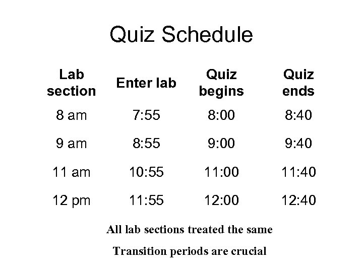Quiz Schedule Lab section Enter lab Quiz begins Quiz ends 8 am 7: 55 8: 00 8: 40 9 am 8: 55 9: 00 9: 40 11 am 10: 55 11: 00 11: 40 12 pm 11: 55 12: 00 12: 40 All lab sections treated the same Transition periods are crucial

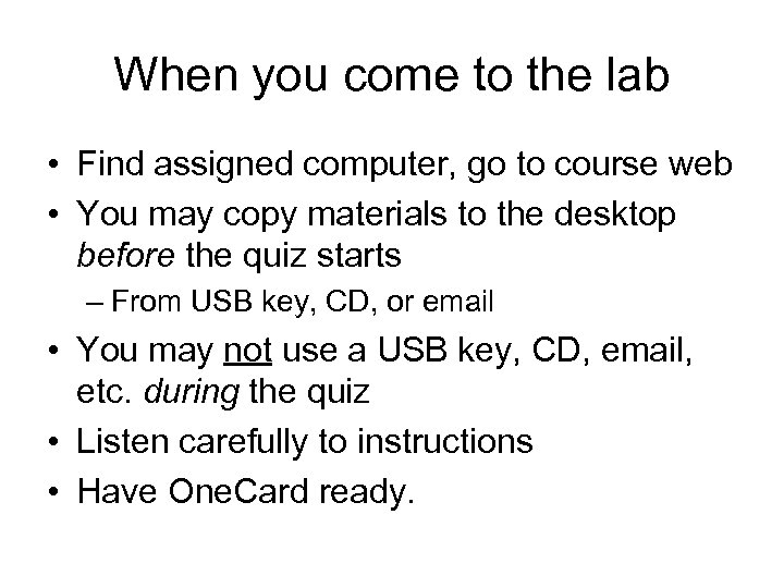When you come to the lab • Find assigned computer, go to course web • You may copy materials to the desktop before the quiz starts – From USB key, CD, or email • You may not use a USB key, CD, email, etc. during the quiz • Listen carefully to instructions • Have One. Card ready.

When the quiz begins • Take a deep breath! • If the first question looks too simple, it is

During the quiz • • • Keep breathing! Save often Submit early, submit often Do not worry about decimals, formatting Later questions may depend on earlier ones. Feel free to make up answers. • If your computer freezes, raise your hand right away. You will be given extra time for computer problems beyond your control.

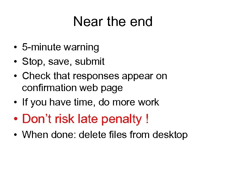Near the end • 5 -minute warning • Stop, save, submit • Check that responses appear on confirmation web page • If you have time, do more work • Don’t risk late penalty ! • When done: delete files from desktop

Things to watch for… • Practice finding good solutions without Solver • Error messages in Solver: – “Error in set target cell not met” – If you see a message you do not recognize, raise your hand immediately and we will help with the tech issue – Do not try to fix this for 20 min and then tell us since we will not be able to give you an extra 20 min on the quiz

Reminders • Quiz Review Session, Thu 5: 30 – 6: 30 pm, BUS B-24+28 – Optional – Q&A session, no new material

MGTSC 352 Lecture 9: Aggregate Planning Overview of Planning: Matching Demand Capacity Case 2: Mountain Wear Leduc Control Example

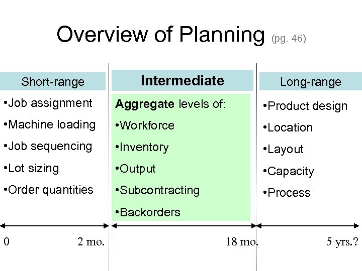Overview of Planning (pg. 46) Short-range Intermediate Long-range • Job assignment Aggregate levels of: • Product design • Machine loading • Workforce • Location • Job sequencing • Inventory • Layout • Lot sizing • Output • Capacity • Order quantities • Subcontracting • Process • Backorders 0 2 mo. 18 mo. 5 yrs. ?

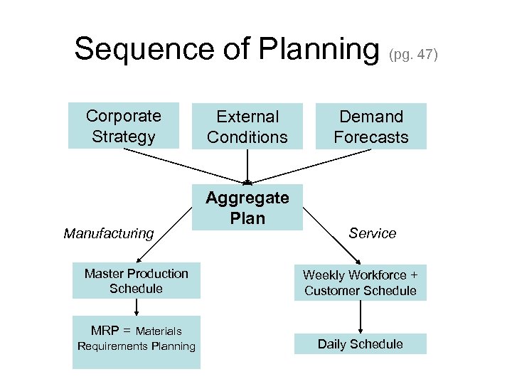Sequence of Planning (pg. 47) Corporate Strategy Manufacturing Master Production Schedule MRP = Materials Requirements Planning External Conditions Aggregate Plan Demand Forecasts Service Weekly Workforce + Customer Schedule Daily Schedule

Matching Demand Capacity Influencing demand • ? Changing capacity • ?

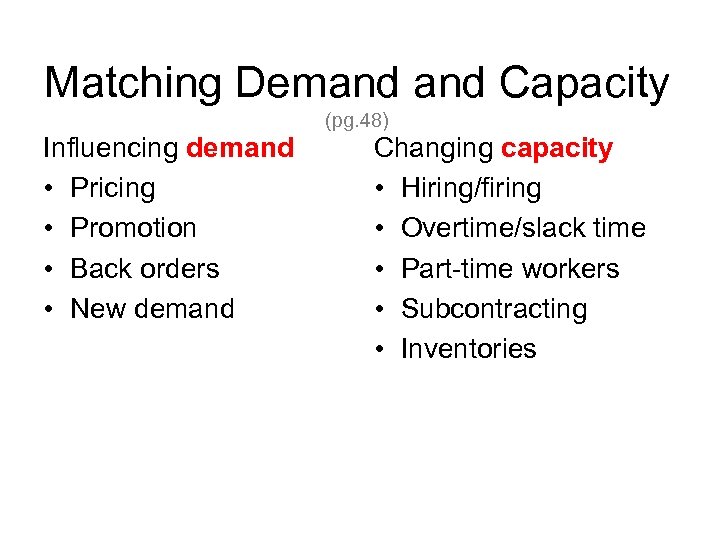Matching Demand Capacity (pg. 48) Influencing demand • Pricing • Promotion • Back orders • New demand Changing capacity • Hiring/firing • Overtime/slack time • Part-time workers • Subcontracting • Inventories

Case 2: Mountain Wear (pg. 96)

Case 2: Mountain Wear Decide … • how much to produce • how much inventory to carry • how many people to hire or lay off • how much overtime to use … in order to satisfy demand minimize cost AGGREGATE PLANNING For next week: read case (pg. 96), fill in the blanks on pages 49 -50 in course pack Let’s look at the first aggregate plan in the case …

Leduc Control (pgs. 52 -53) • The mysteries of solver unraveled … – … slowly • How many units of each product to produce for the next period? – Simpler than Mountain Wear

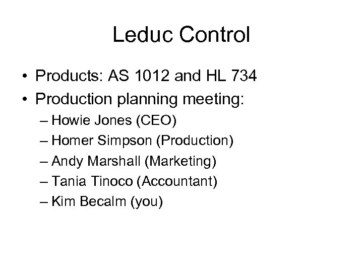Leduc Control • Products: AS 1012 and HL 734 • Production planning meeting: – Howie Jones (CEO) – Homer Simpson (Production) – Andy Marshall (Marketing) – Tania Tinoco (Accountant) – Kim Becalm (you)

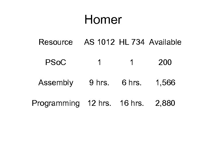Homer Resource AS 1012 HL 734 Available PSo. C 1 1 200 Assembly 9 hrs. 6 hrs. 1, 566 Programming 12 hrs. 16 hrs. 2, 880

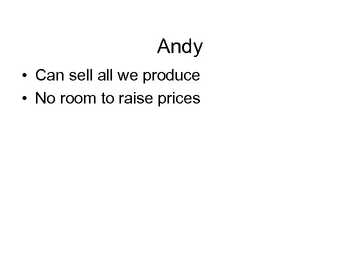Andy • Can sell all we produce • No room to raise prices

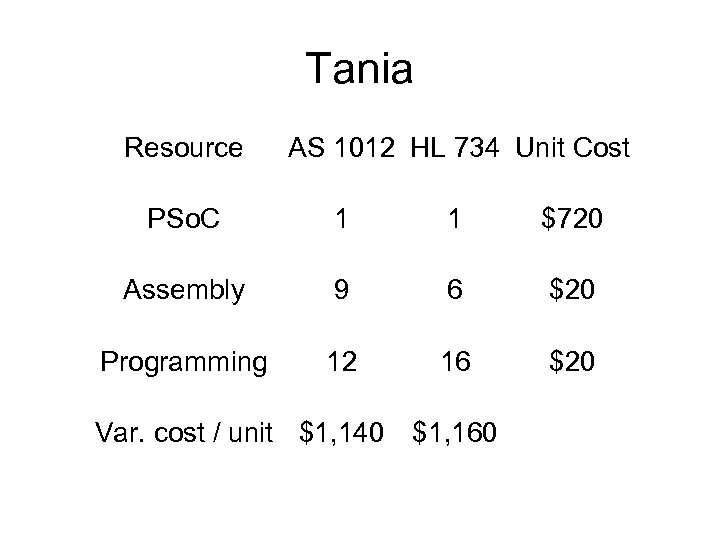Tania Resource AS 1012 HL 734 Unit Cost PSo. C 1 1 $720 Assembly 9 6 $20 Programming 12 16 $20 Var. cost / unit $1, 140 $1, 160

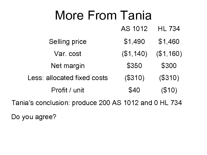More From Tania AS 1012 HL 734 Selling price $1, 490 $1, 460 Var. cost ($1, 140) ($1, 160) Net margin $350 $300 Less: allocated fixed costs ($310) Profit / unit $40 ($10) Tania’s conclusion: produce 200 AS 1012 and 0 HL 734 Do you agree?

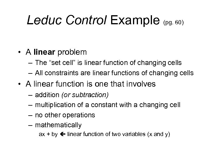Leduc Control Example (pg. 60) • A linear problem – The “set cell” is linear function of changing cells – All constraints are linear functions of changing cells • A linear function is one that involves – – addition (or subtraction) multiplication of a constant with a changing cell no other operations mathematically ax + by linear function of two variables (x and y)

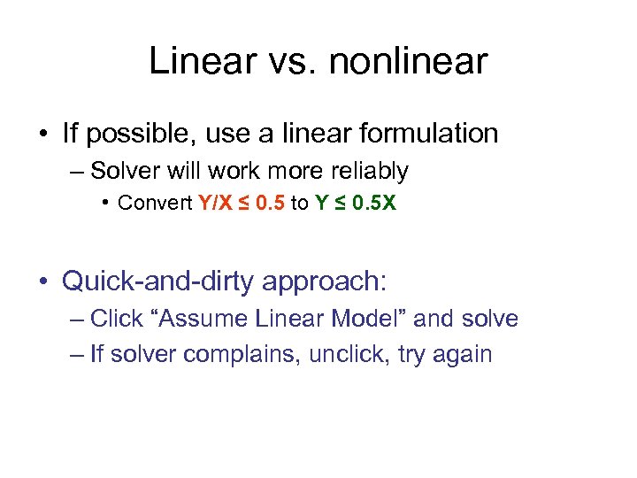Linear vs. nonlinear • If possible, use a linear formulation – Solver will work more reliably • Convert Y/X ≤ 0. 5 to Y ≤ 0. 5 X • Quick-and-dirty approach: – Click “Assume Linear Model” and solve – If solver complains, unclick, try again

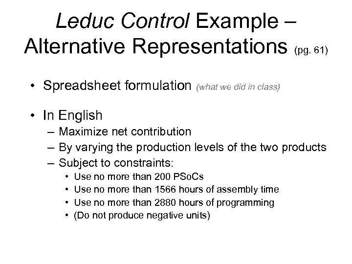Leduc Control Example – Alternative Representations (pg. 61) • Spreadsheet formulation (what we did in class) • In English – Maximize net contribution – By varying the production levels of the two products – Subject to constraints: • • Use no more than 200 PSo. Cs Use no more than 1566 hours of assembly time Use no more than 2880 hours of programming (Do not produce negative units)

Algebraic Formulation

Matrix Formulation

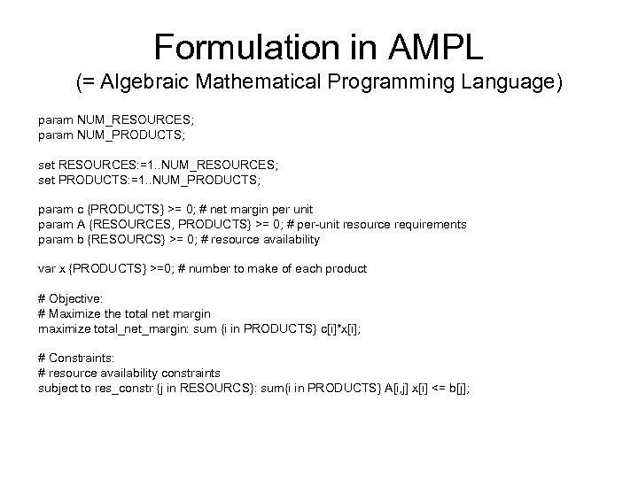Formulation in AMPL (= Algebraic Mathematical Programming Language) param NUM_RESOURCES; param NUM_PRODUCTS; set RESOURCES: =1. . NUM_RESOURCES; set PRODUCTS: =1. . NUM_PRODUCTS; param c {PRODUCTS} >= 0; # net margin per unit param A {RESOURCES, PRODUCTS} >= 0; # per-unit resource requirements param b {RESOURCS} >= 0; # resource availability var x {PRODUCTS} >=0; # number to make of each product # Objective: # Maximize the total net margin maximize total_net_margin: sum {i in PRODUCTS} c[i]*x[i]; # Constraints: # resource availability constraints subject to res_constr {j in RESOURCS}: sum{i in PRODUCTS} A[i, j] x[i] <= b[j];

Which Formulation is Best? • Depends on what you want to do: – Understand the problem – Solve the problem • Small problem • Big problem – Communicate the problem – Develop a new/improved solver

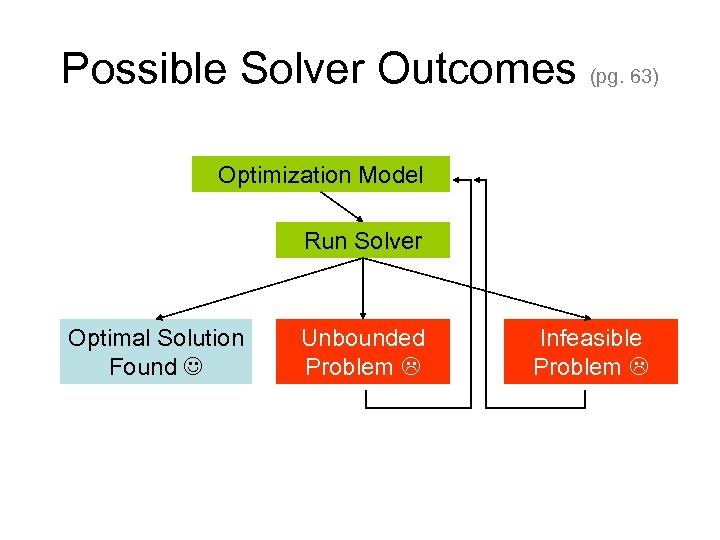Possible Solver Outcomes (pg. 63) Optimization Model Run Solver Optimal Solution Found Unbounded Problem Infeasible Problem

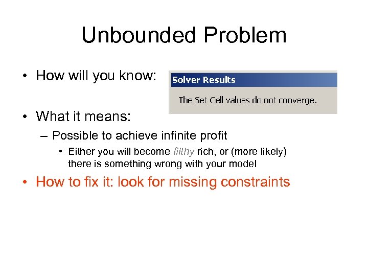Unbounded Problem • How will you know: • What it means: – Possible to achieve infinite profit • Either you will become filthy rich, or (more likely) there is something wrong with your model • How to fix it: look for missing constraints

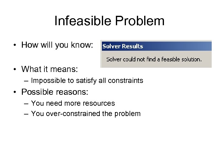Infeasible Problem • How will you know: • What it means: – Impossible to satisfy all constraints • Possible reasons: – You need more resources – You over-constrained the problem

Unbounded/Infeasible Problem • Means solver cannot solve • The values returned are meaningless – You need to look at your model

Is the plan still optimal? If not, how will it change? (pg. 65) 1. Howie realizes that he underestimated the net margin for each AS by $65. 2. Howie realizes that he overestimated the net margin for each AS by $65. 3. Howie discovers a new market where he can sell both AS and HLs at a 20% higher net margin than originally estimated.

More Post-Optimality Analysis 4. Another semiconductor supplier offers Howie 5 more Pso. Cs for a premium of $150 each (above and beyond the going rate of $720 per unit). Should Howie buy these PSo. Cs? 5. Howie sometimes helps out with programming the LCDs, thereby increasing the amount of available programming time. Should he help out in this cycle? If so, how long should he help out? 6. Howie’s nephew offers to work in assembly for a premium rate of $12 per hour (above and beyond the going rate of $20 per hour). Should Howie hire his nephew? For how many hours?

Solver. Table (pg. 67) • Combines Solver and Data Table • Solves the problem repeatedly and reports all solutions • Free add-in – see COURSE DOCUMENTS > RESOURCES > SOFTWARE on course web

Excel Solver Advantages (pg. 69) • comes with Excel (no additional cost) • has the same familiar user interface as other Excel components • can solve problems with integer constraints and nonlinear problems • can be automated using VBA

Excel Solver Disadvantages • limited to 200 variables and 100 constraints (Premium: 800 variables, no limit on constraints) • somewhat inconvenient (Ex: B 12 + B 13 ≤ B 14 not allowed) • can be slow when solving large problems with integer constraints (Premium Solver much faster) • not very reliable (sometimes fails to find a solution) (Premium is more robust)

Other solvers • Survey – http: //lionhrtpub. com/orms/surveys/LP/LP-survey. html • $1, 000. . . $10, 000 • Can solve very large problems (200, 000 constraints) • Usually require front-end modeling language • Premium solver: $1, 000 http: //www. solver. com/