Predictive Learning from Data LECTURE SET 4 Statistical

Predictive Learning from Data LECTURE SET 4 Statistical Learning Theory (VC-theory) Electrical and Computer Engineering 1

OUTLINE • Objectives • Inductive learning problem setting • Statistical Learning Theory • Applications • Measuring the VC-dimension • Summary and discussion 2

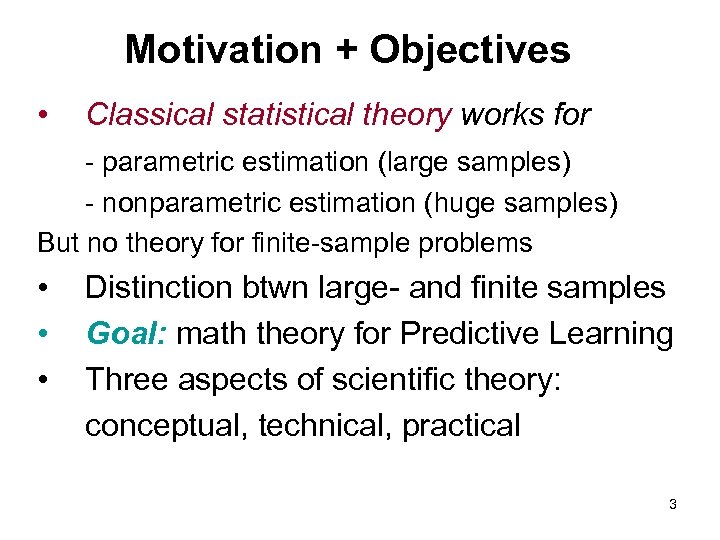Motivation + Objectives • Classical statistical theory works for - parametric estimation (large samples) - nonparametric estimation (huge samples) But no theory for finite-sample problems • • • Distinction btwn large- and finite samples Goal: math theory for Predictive Learning Three aspects of scientific theory: conceptual, technical, practical 3

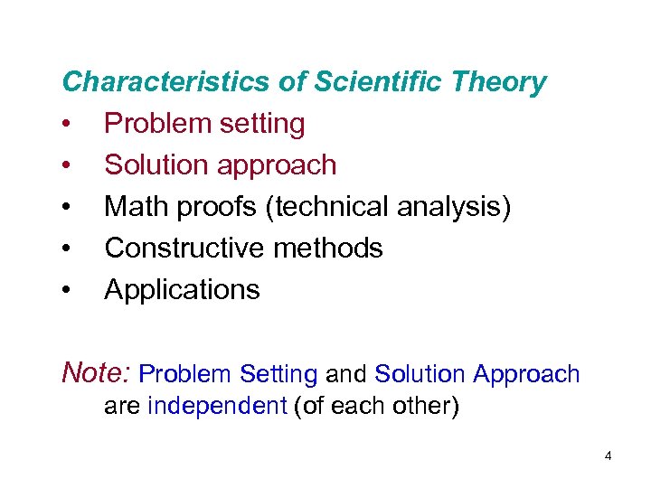Characteristics of Scientific Theory • Problem setting • Solution approach • Math proofs (technical analysis) • Constructive methods • Applications Note: Problem Setting and Solution Approach are independent (of each other) 4

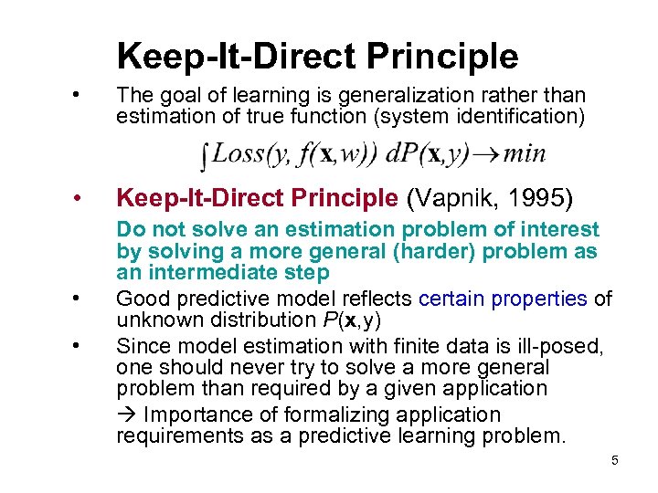Keep-It-Direct Principle • The goal of learning is generalization rather than estimation of true function (system identification) • Keep-It-Direct Principle (Vapnik, 1995) • • Do not solve an estimation problem of interest by solving a more general (harder) problem as an intermediate step Good predictive model reflects certain properties of unknown distribution P(x, y) Since model estimation with finite data is ill-posed, one should never try to solve a more general problem than required by a given application Importance of formalizing application requirements as a predictive learning problem. 5

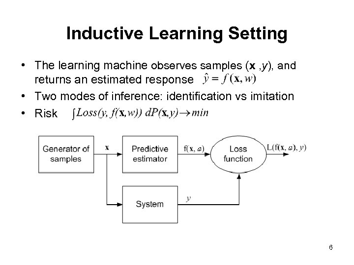Inductive Learning Setting • The learning machine observes samples (x , y), and returns an estimated response • Two modes of inference: identification vs imitation • Risk 6

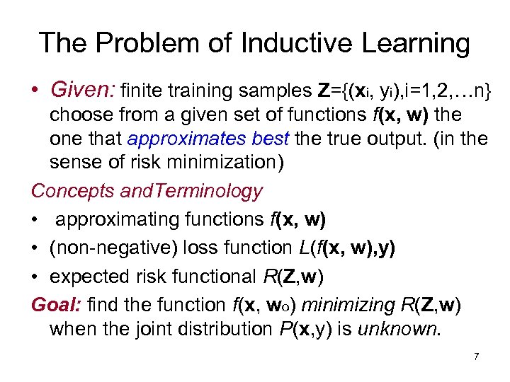The Problem of Inductive Learning • Given: finite training samples Z={(xi, yi), i=1, 2, …n} choose from a given set of functions f(x, w) the one that approximates best the true output. (in the sense of risk minimization) Concepts and. Terminology • approximating functions f(x, w) • (non-negative) loss function L(f(x, w), y) • expected risk functional R(Z, w) Goal: find the function f(x, wo) minimizing R(Z, w) when the joint distribution P(x, y) is unknown. 7

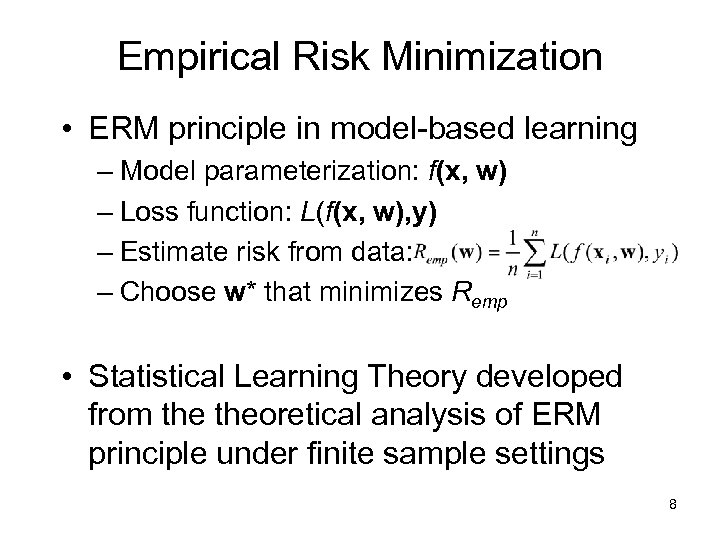Empirical Risk Minimization • ERM principle in model-based learning – Model parameterization: f(x, w) – Loss function: L(f(x, w), y) – Estimate risk from data: – Choose w* that minimizes Remp • Statistical Learning Theory developed from theoretical analysis of ERM principle under finite sample settings 8

OUTLINE • Objectives • Inductive learning problem setting • Statistical Learning Theory • Applications • Measuring the VC-dimension • Summary and discussion 9

Statistical Learning Theory • History and Overview • Conditions for consistency and convergence of ERM • VC-dimension • Generalization bounds • Structural Risk Minimization (SRM) for learning with finite samples 10

History and Overview • SLT aka VC-theory (Vapnik-Chervonenkis) • Theory for estimating dependencies from finite samples (predictive learning setting) • Based on the risk minimization approach • All main results originally developed in 1970’s for classification (pattern recognition) – why? but remained largely unknown • Renewed interest since late 90’s due to practical success of Support Vector Machines (SVM) 11

History and Overview(cont’d) MAIN CONTRIBUTIONS • Distinction between problem setting, inductive principle and learning algorithms • Direct approach to estimation with finite data (KID principle) • Math analysis of ERM (inductive setting) • Two factors responsible for generalization: - empirical risk (fitting/ training error) - complexity(capacity) of approximating functions 12

History and Overview(cont’d) VC-theory has 4 parts: 1. Conditions for consistency/ convergence of ERM 2. Generalization bounds 3. Inductive principles (for finite samples) 4. Constructive methods (learning algorithms) for implementing (3) NOTE: (1) (2) (3) (4) 13

Consistency/Convergence of ERM • Empirical Risk known but Expected Risk unknown • Asymptotic consistency requirement: under what (general) conditions models providing min Empirical Risk will also provide min Prediction Risk, when the number of samples grows large? • Why asymptotic analysis is important? - helps to develop useful concepts - necessary and sufficient conditions ensure that VC-theory is general and cannot be improved 14

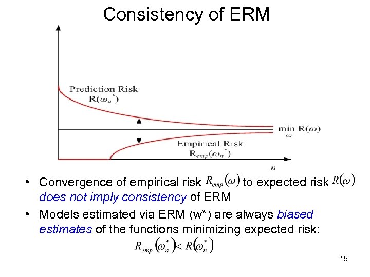Consistency of ERM • Convergence of empirical risk to expected risk does not imply consistency of ERM • Models estimated via ERM (w*) are always biased estimates of the functions minimizing expected risk: 15

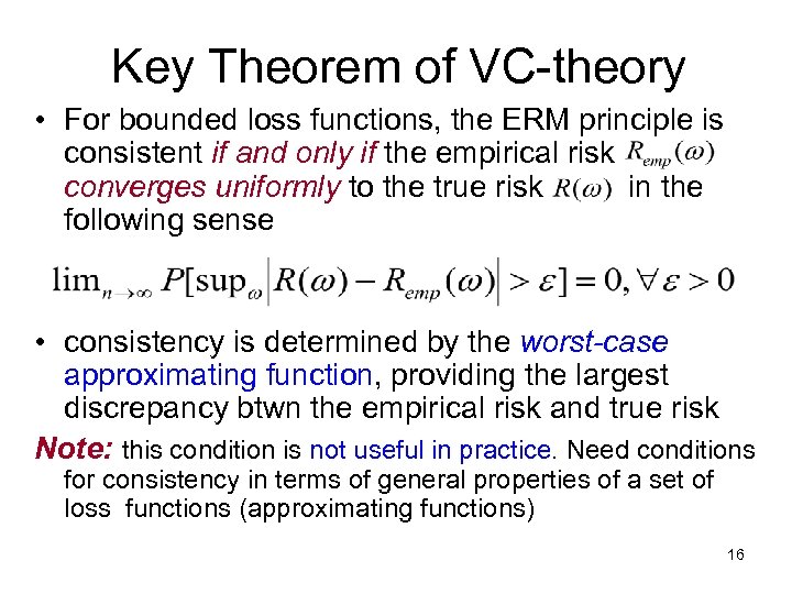Key Theorem of VC-theory • For bounded loss functions, the ERM principle is consistent if and only if the empirical risk converges uniformly to the true risk in the following sense • consistency is determined by the worst-case approximating function, providing the largest discrepancy btwn the empirical risk and true risk Note: this condition is not useful in practice. Need conditions for consistency in terms of general properties of a set of loss functions (approximating functions) 16

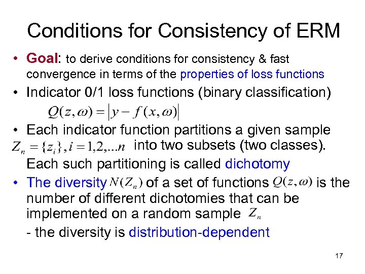Conditions for Consistency of ERM • Goal: to derive conditions for consistency & fast convergence in terms of the properties of loss functions • Indicator 0/1 loss functions (binary classification) • Each indicator function partitions a given sample into two subsets (two classes). Each such partitioning is called dichotomy • The diversity of a set of functions is the number of different dichotomies that can be implemented on a random sample - the diversity is distribution-dependent 17

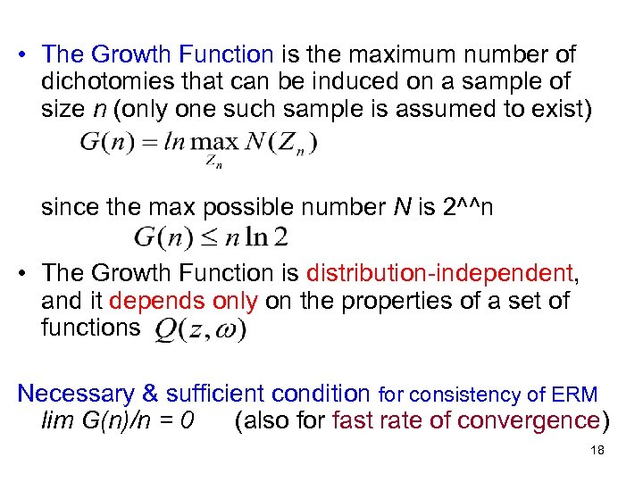• The Growth Function is the maximum number of dichotomies that can be induced on a sample of size n (only one such sample is assumed to exist) since the max possible number N is 2^^n • The Growth Function is distribution-independent, and it depends only on the properties of a set of functions Necessary & sufficient condition for consistency of ERM lim G(n)/n = 0 (also for fast rate of convergence) 18

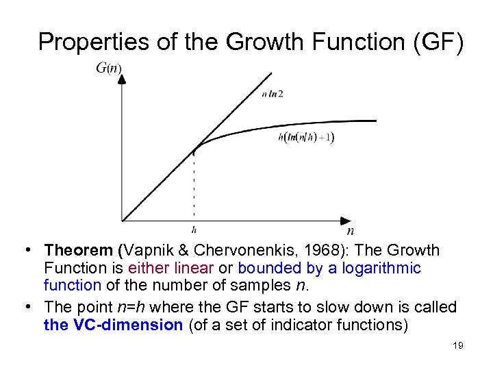Properties of the Growth Function (GF) • Theorem (Vapnik & Chervonenkis, 1968): The Growth Function is either linear or bounded by a logarithmic function of the number of samples n. • The point n=h where the GF starts to slow down is called the VC-dimension (of a set of indicator functions) 19

VC-dimension • If the bound on the GF stays linear for any n: G(n) = n ln 2 then the VC-dimension is infinite lim G(n)/n = ln 2 and the ERM is inconsistent. That is, any sample of size n can be split in 2^^n possible ways; hence no valid generalization is possible • Necessary and sufficient condition for consistency of ERM: Vapnik-Chervonenkis (VC) dimension is finite (this condition is distribution-independent) 20

• VC-dimension measures the ability (of a set of functions) to fit or ‘explain’ available finite data. • VC-dimension of a set of indicator functions: - Shattering: if n samples can be separated by a set of indicator functions in all 2^^n possible ways, then these samples can be shattered by this set of functions. - A set of functions has VC-dimension h if there exist h samples that can be shattered by this set of functions, but there does not exist h+1 samples that can be shattered. • Examples of analytic calculation of VC-dimension for simple sets of functions are shown next 21

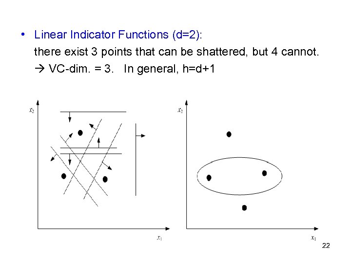• Linear Indicator Functions (d=2): there exist 3 points that can be shattered, but 4 cannot. VC-dim. = 3. In general, h=d+1 22

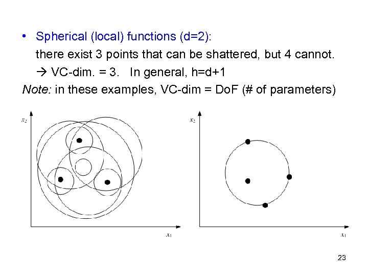• Spherical (local) functions (d=2): there exist 3 points that can be shattered, but 4 cannot. VC-dim. = 3. In general, h=d+1 Note: in these examples, VC-dim = Do. F (# of parameters) 23

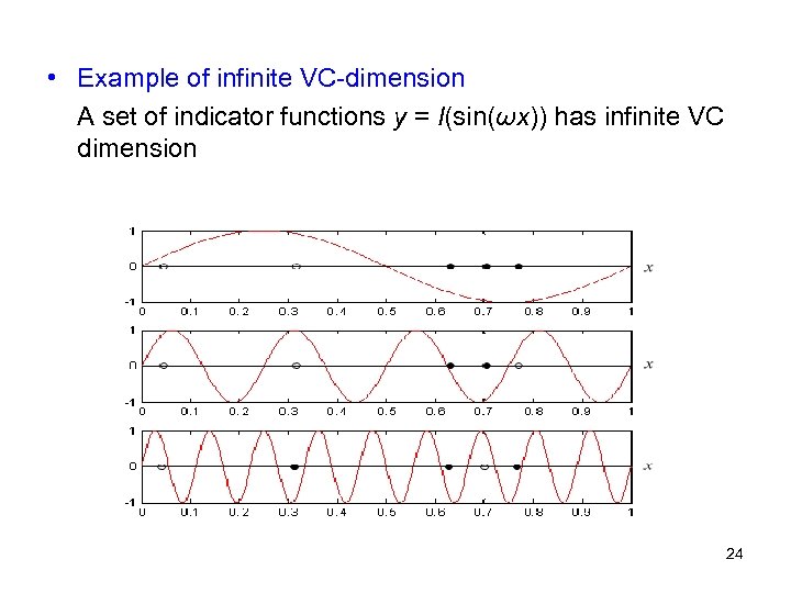• Example of infinite VC-dimension A set of indicator functions y = I(sin(ωx)) has infinite VC dimension 24

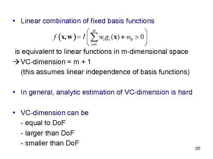• Linear combination of fixed basis functions is equivalent to linear functions in m-dimensional space VC-dimension = m + 1 (this assumes linear independence of basis functions) • In general, analytic estimation of VC-dimension is hard • VC-dimension can be - equal to Do. F - larger than Do. F - smaller than Do. F 25

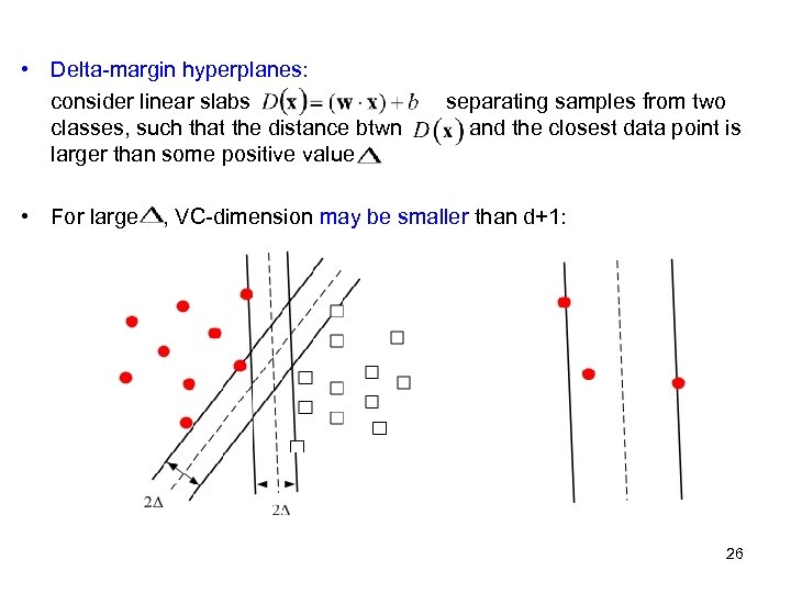• Delta-margin hyperplanes: consider linear slabs classes, such that the distance btwn larger than some positive value • For large separating samples from two and the closest data point is , VC-dimension may be smaller than d+1: 26

VC-dimension and Falsifiability • A set of functions has VC-dimension h if (a) It can explain (shatter) a set of h samples ~ there exists h samples that cannot falsify it and (b) It can not shatter h+1 samples ~ any h+1 samples falsify this set • Finiteness of VC-dim is necessary and sufficient condition for generalization (for any learning method based on ERM) 27

Philosophical interpretation: VCfalsifiability • Occam’s Razor: Select the model that explains available data and has the smallest number of free parameters (entities) • VC theory: Select the model that explains available data and has low VC-dimension (i. e. can be easily falsified) New principle of VC falsifiability 28

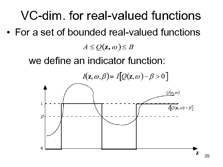VC-dim. for real-valued functions • For a set of bounded real-valued functions we define an indicator function: 29

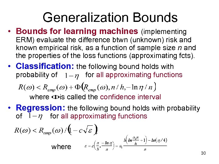Generalization Bounds • Bounds for learning machines (implementing ERM) evaluate the difference btwn (unknown) risk and known empirical risk, as a function of sample size n and the properties of the loss functions (approximating fcts). • Classification: the following bound holds with probability of where for all approximating functions is called the confidence interval • Regression: the following bound holds with probability of for all approximating functions where 30

COMMENTS ON VC-BOUNDS • Useful for conceptual understanding of general properties & limitations of all learning methods • Not appropriate for practical use • Properties of VC-bounds: - the confidence interval monotonically decreases to zero (with n) - bounds depend strongly on n/h; - bounds do not depend on dimensionality 31

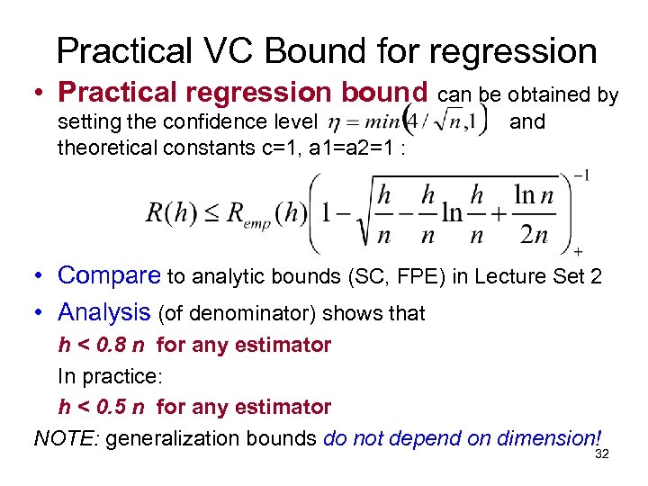Practical VC Bound for regression • Practical regression bound can be obtained by setting the confidence level theoretical constants c=1, a 1=a 2=1 : and • Compare to analytic bounds (SC, FPE) in Lecture Set 2 • Analysis (of denominator) shows that h < 0. 8 n for any estimator In practice: h < 0. 5 n for any estimator NOTE: generalization bounds do not depend on dimension! 32

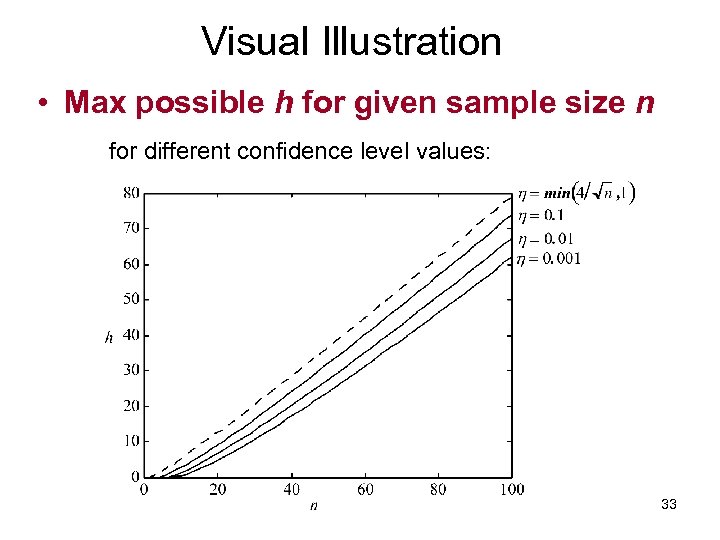Visual Illustration • Max possible h for given sample size n for different confidence level values: 33

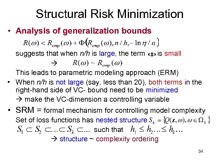Structural Risk Minimization • Analysis of generalization bounds suggests that when n/h is large, the term is small This leads to parametric modeling approach (ERM) • When n/h is not large (say, less than 20), both terms in the right-hand side of VC- bound need to be minimized make the VC-dimension a controlling variable • SRM = formal mechanism for controlling model complexity Set of loss functions has nested structure such that structure ~ complexity ordering 34

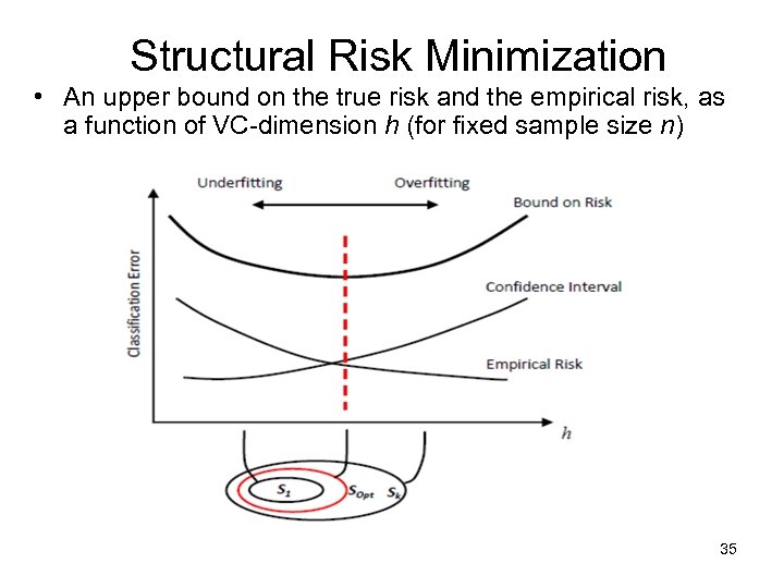Structural Risk Minimization • An upper bound on the true risk and the empirical risk, as a function of VC-dimension h (for fixed sample size n) 35

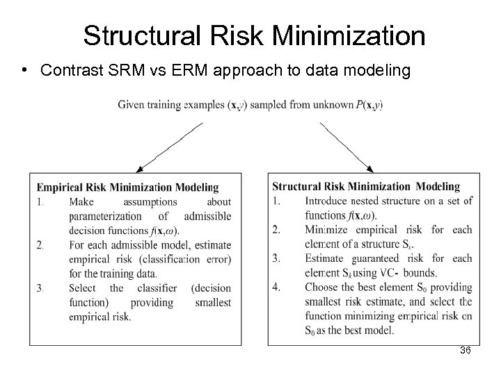Structural Risk Minimization • Contrast SRM vs ERM approach to data modeling 36

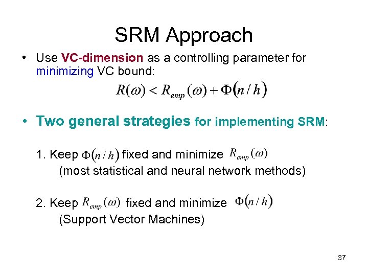SRM Approach • Use VC-dimension as a controlling parameter for minimizing VC bound: • Two general strategies for implementing SRM: 1. Keep fixed and minimize (most statistical and neural network methods) 2. Keep fixed and minimize (Support Vector Machines) 37

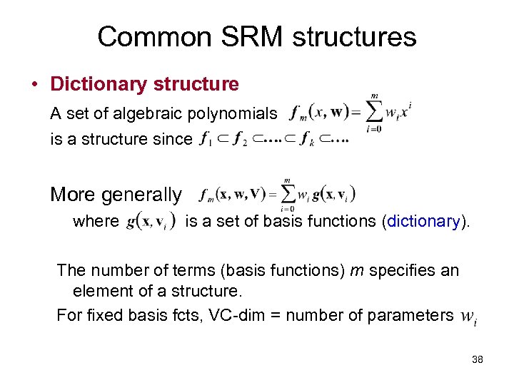Common SRM structures • Dictionary structure A set of algebraic polynomials is a structure since More generally where is a set of basis functions (dictionary). The number of terms (basis functions) m specifies an element of a structure. For fixed basis fcts, VC-dim = number of parameters 38

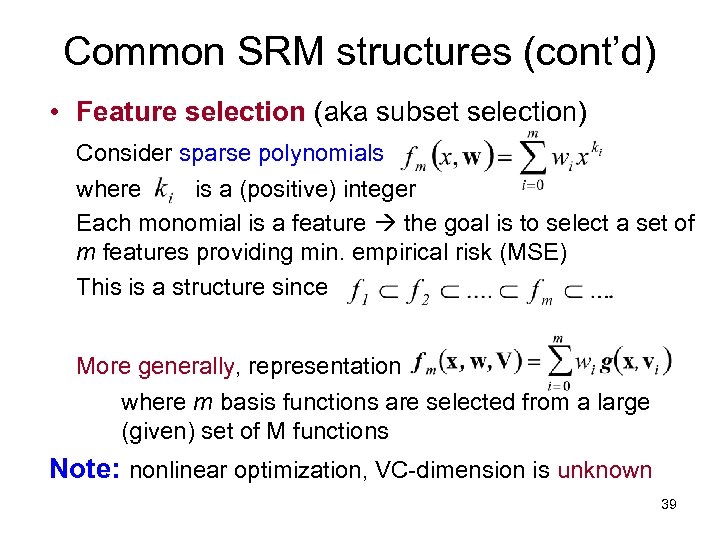Common SRM structures (cont’d) • Feature selection (aka subset selection) Consider sparse polynomials where is a (positive) integer Each monomial is a feature the goal is to select a set of m features providing min. empirical risk (MSE) This is a structure since More generally, representation where m basis functions are selected from a large (given) set of M functions Note: nonlinear optimization, VC-dimension is unknown 39

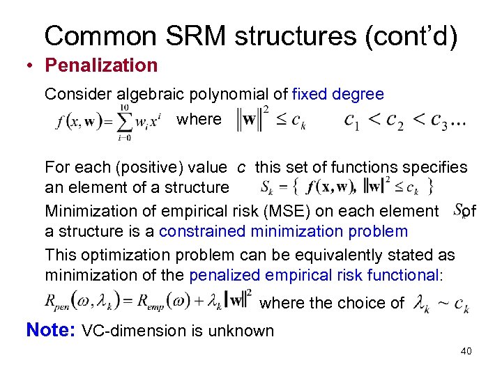Common SRM structures (cont’d) • Penalization Consider algebraic polynomial of fixed degree where For each (positive) value c this set of functions specifies an element of a structure Minimization of empirical risk (MSE) on each element of a structure is a constrained minimization problem This optimization problem can be equivalently stated as minimization of the penalized empirical risk functional: where the choice of Note: VC-dimension is unknown 40

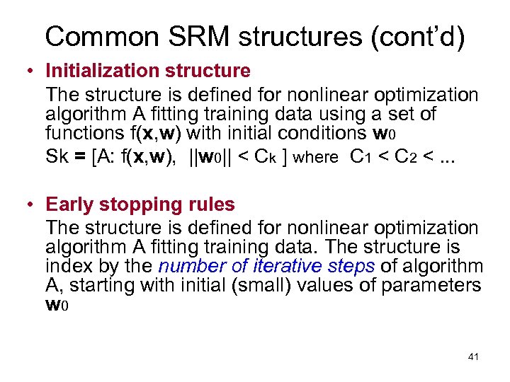Common SRM structures (cont’d) • Initialization structure The structure is defined for nonlinear optimization algorithm A fitting training data using a set of functions f(x, w) with initial conditions w 0 Sk = [A: f(x, w), ||w 0|| < Ck ] where C 1 < C 2 <. . . • Early stopping rules The structure is defined for nonlinear optimization algorithm A fitting training data. The structure is index by the number of iterative steps of algorithm A, starting with initial (small) values of parameters w 0 41

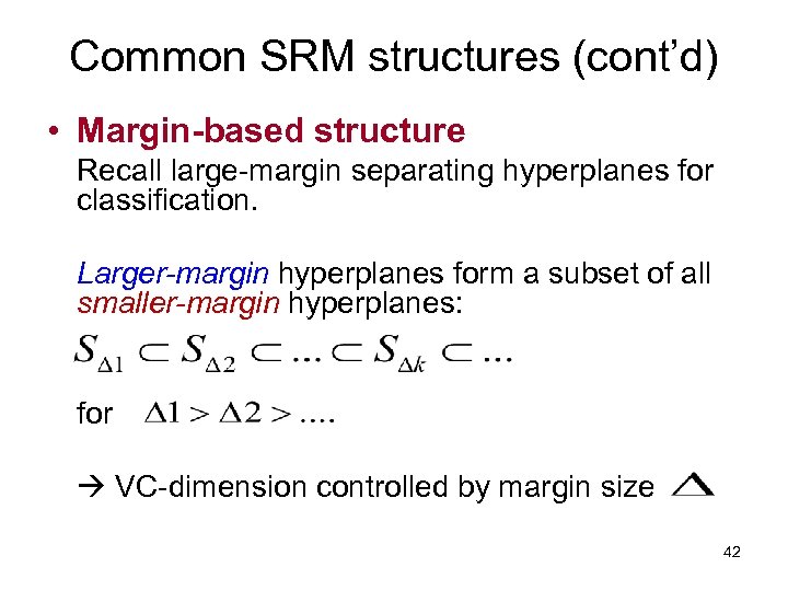Common SRM structures (cont’d) • Margin-based structure Recall large-margin separating hyperplanes for classification. Larger-margin hyperplanes form a subset of all smaller-margin hyperplanes: for VC-dimension controlled by margin size 42

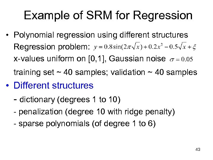Example of SRM for Regression • Polynomial regression using different structures Regression problem: x-values uniform on [0, 1], Gaussian noise training set ~ 40 samples; validation ~ 40 samples • Different structures - dictionary (degrees 1 to 10) - penalization (degree 10 with ridge penalty) - sparse polynomials (of degree 1 to 6) 43

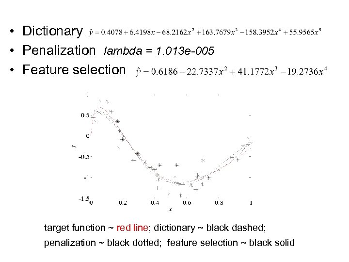• Dictionary • Penalization lambda = 1. 013 e-005 • Feature selection target function ~ red line; dictionary ~ black dashed; penalization ~ black dotted; feature selection ~ black solid 44

Aside: model interpretation • Outside the scope of VC-theory • In the last example: different structures on the same set of functions lead to different interpretations • Often interpretation assumes function identification setting • In practice, interpretation always requires application domain knowledge 45

Practical Implementation of SRM • Need to - estimate VC-dim for an element of a structure Sk - minimize empirical risk for each element Sk • Both possible for linear approximating functions • Both difficult for nonlinear parameterization many heuristic learning algorithms 46

SRM structures: summary • SRM structure ~ complexity ordering on a set of admissible models (approximating functions) • Many different structures on the same set of approximating functions Which one is the ‘best’? - depends on the properties of application data - can be decided via empirical comparisons • SRM = mechanism for complexity control - selecting optimal complexity for a given data set - new measure of complexity: VC-dimension - model selection using analytic VC-bounds 47

OUTLINE • • • Objectives Inductive learning problem setting Statistical Learning Theory Applications - model selection (for regression) - market timing of international funds - signal denoising Measuring the VC-dimension Summary and discussion 48

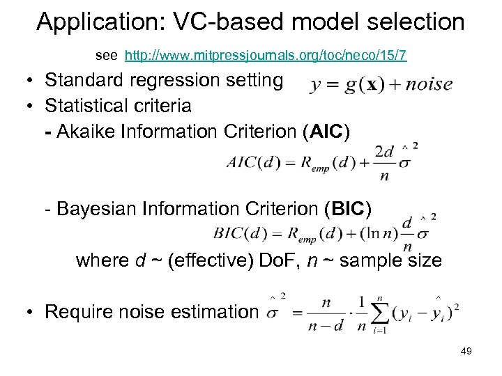Application: VC-based model selection see http: //www. mitpressjournals. org/toc/neco/15/7 • Standard regression setting • Statistical criteria - Akaike Information Criterion (AIC) - Bayesian Information Criterion (BIC) where d ~ (effective) Do. F, n ~ sample size • Require noise estimation 49

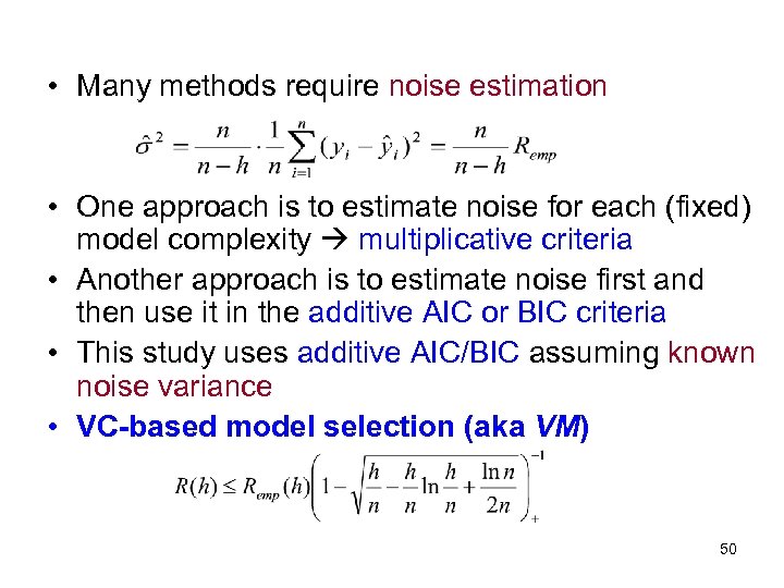• Many methods require noise estimation • One approach is to estimate noise for each (fixed) model complexity multiplicative criteria • Another approach is to estimate noise first and then use it in the additive AIC or BIC criteria • This study uses additive AIC/BIC assuming known noise variance • VC-based model selection (aka VM) 50

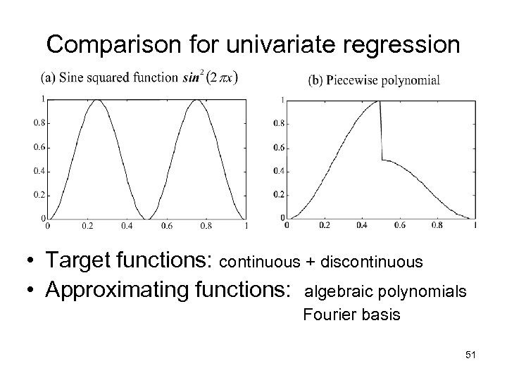Comparison for univariate regression • Target functions: continuous + discontinuous • Approximating functions: algebraic polynomials Fourier basis 51

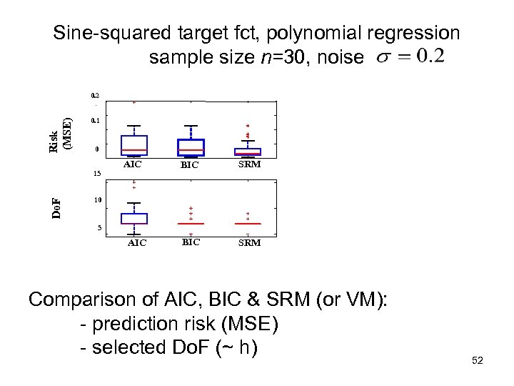Sine-squared target fct, polynomial regression sample size n=30, noise Risk (MSE) 0. 2 0. 1 0 AIC Do. F 15 BIC SRM 10 5 AIC Comparison of AIC, BIC & SRM (or VM): - prediction risk (MSE) - selected Do. F (~ h) 52

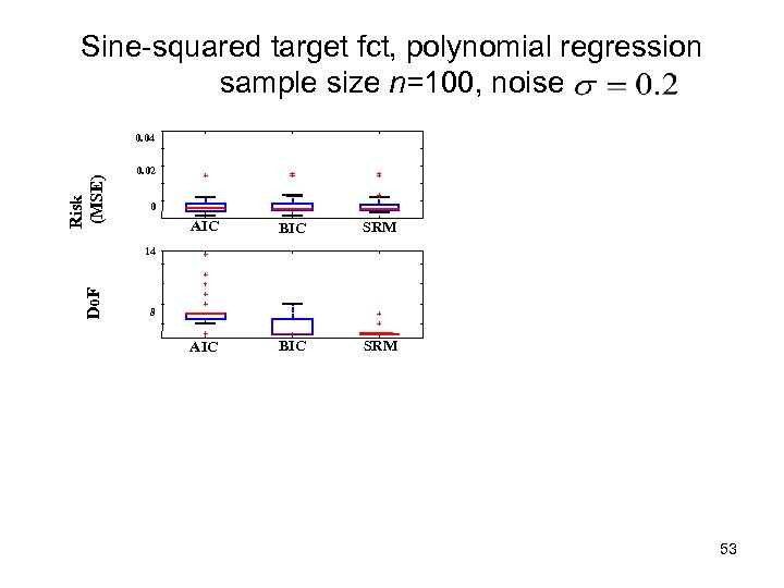Sine-squared target fct, polynomial regression sample size n=100, noise Risk (MSE) 0. 04 0. 02 0 AIC BIC SRM Do. F 14 8 53

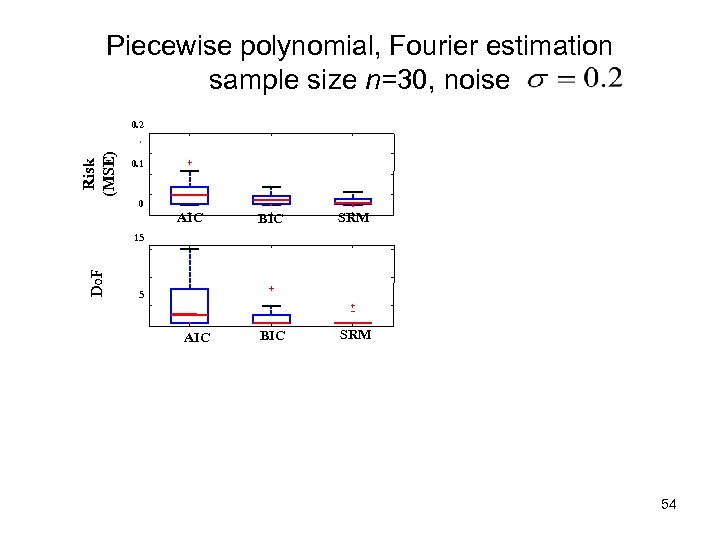Piecewise polynomial, Fourier estimation sample size n=30, noise Risk (MSE) 0. 2 0. 1 0 AIC BIC SRM Do. F 15 5 AIC 54

Comparison for linear subset selection • Target function: • x-values uniform in [0, 1], n=30 samples gaussian noise • Approximating functions: linear subset selection Risk (MSE) 0. 04 0. 02 0 AIC BIC vm Do. F 6 4 2 55

Lots of confusion about model selection • Cherkassky et al (1999): VC-analytic bound works very well for (univariate) regression problems Hastie et al (2001): SRM (using VC-bound) performs poorly overall See http: //www. mitpressjournals. org/toc/neco/15/7 • What is the cause for disagreement? - technical sloppiness + lack of common sense • More confusing studies are generated each year See http: //www. springerlink. com/content/kq 4 g 614 j 3 xhdupuu/fullt ext. pdf Discussion question: read the paper Sugiama & Ogawa(2002) and try to understand the deficiencies in their experimental procedure and/or assumptions used in this paper. 56

Market Timing of International Funds: A Decade after the Scandal Vladimir Cherkassky and Sauptik Dhar University of Minnesota cherk 001@umn. edu Presented at CIFEr, March 30, 2012 Electrical and Computer Engineering 57

OUTLINE • Motivation + Background - mutual fund basics - scandals in early 2000’s - regulations on frequent trading • • • Predictive (VC-theoretical) methodology Empirical Results: market timing of TWIEX Conclusions and policy implications 58

Timing of International Funds • International mutual funds - priced at 4 pm EST - reflect price of foreign securities traded at European/ Asian markets - Foreign markets close earlier than US market Possibility of inefficient pricing Market timing exploits this inefficiency. • Logical solution: implement efficient pricing [ Zitzewitz 2003] • Solution adopted: restrictions on trading 59

Data Analytic Approach • Timing of international mutual funds Can it be consistently profitable under - past market conditions ? (2004 ~ 2005) - current market conditions ? (2009 ~ 2012) • • Predictive data modeling: - estimate trading model (using past data) - apply this model for prediction (trading) Diversified international fund (TWIEX) American Century Int’l Growth Fund 60

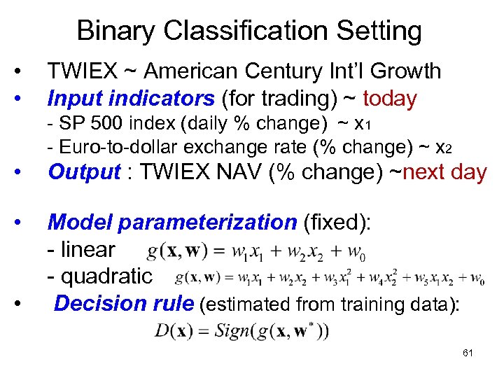Binary Classification Setting • • TWIEX ~ American Century Int’l Growth Input indicators (for trading) ~ today - SP 500 index (daily % change) ~ x 1 - Euro-to-dollar exchange rate (% change) ~ x 2 • Output : TWIEX NAV (% change) ~next day • Model parameterization (fixed): - linear - quadratic Decision rule (estimated from training data): • 61

VC theoretical Methodology • When a trained model can predict well? (1) Future/test data is similar to training data i. e. , use 2004 period for training, and 2005 for testing (2) Estimated model is ‘simple’ and provides good performance during training period i. e. , trading strategy is consistently better than buy-and-hold during training period 62

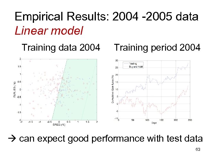Empirical Results: 2004 -2005 data Linear model Training data 2004 Training period 2004 can expect good performance with test data 63

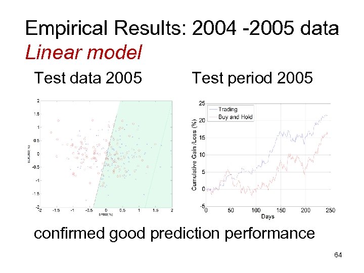Empirical Results: 2004 -2005 data Linear model Test data 2005 Test period 2005 confirmed good prediction performance 64

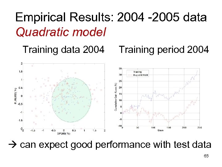Empirical Results: 2004 -2005 data Quadratic model Training data 2004 Training period 2004 can expect good performance with test data 65

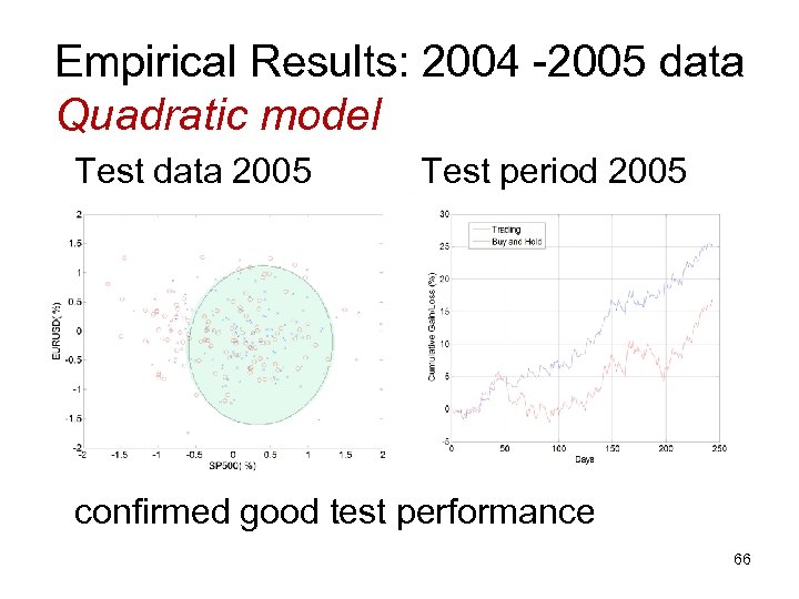Empirical Results: 2004 -2005 data Quadratic model Test data 2005 Test period 2005 confirmed good test performance 66

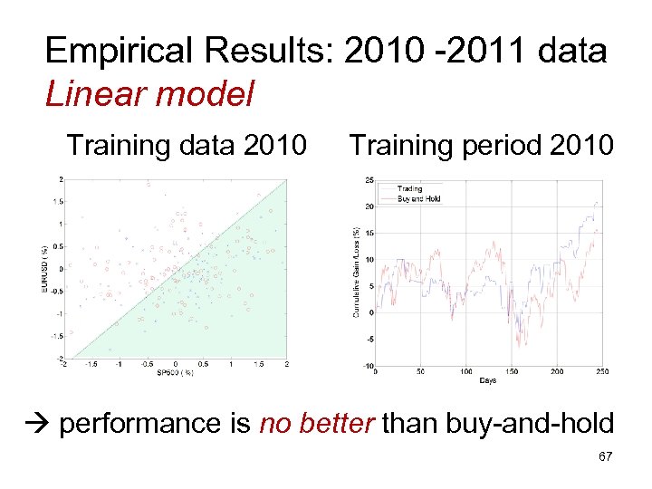Empirical Results: 2010 -2011 data Linear model Training data 2010 Training period 2010 performance is no better than buy-and-hold 67

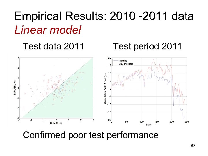Empirical Results: 2010 -2011 data Linear model Test data 2011 Test period 2011 Confirmed poor test performance 68

Summary of Results for TWIEX • • Market timing worked well during past market conditions (i. e. , 2004 – 2005 period) Market timing does not work under current market conditions (i. e. , 2008 – 2012 period) Similar conclusions hold for - other international mutual funds - other time periods (say prior to 2004) Explanation: statistical characteristics of the stock market have changed 69

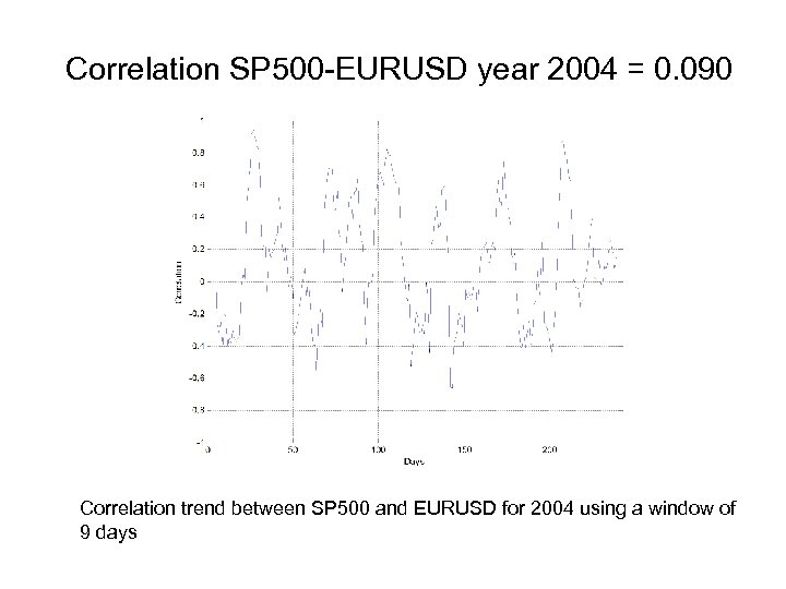Correlation SP 500 -EURUSD year 2004 = 0. 090 Correlation trend between SP 500 and EURUSD for 2004 using a window of 9 days

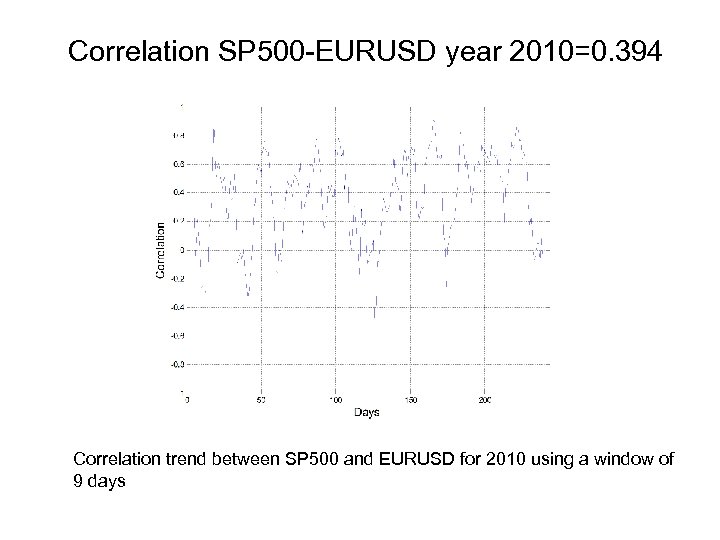Correlation SP 500 -EURUSD year 2010=0. 394 Correlation trend between SP 500 and EURUSD for 2010 using a window of 9 days

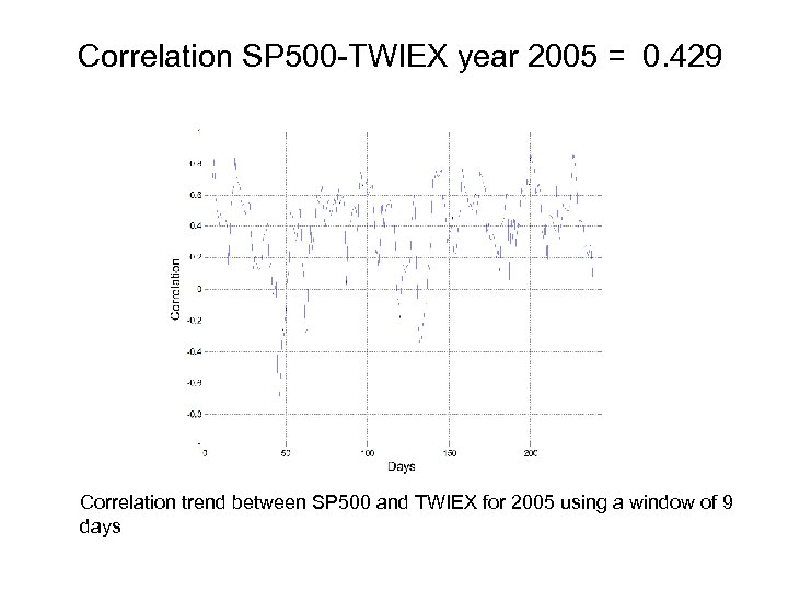Correlation SP 500 -TWIEX year 2005 = 0. 429 Correlation trend between SP 500 and TWIEX for 2005 using a window of 9 days

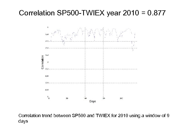Correlation SP 500 -TWIEX year 2010 = 0. 877 Correlation trend between SP 500 and TWIEX for 2010 using a window of 9 days

Aside: Interpretation vs Prediction • • • Interpretation: outside the scope of VCtheory Only prediction can be objectively evaluated Multiplicity of good predictive models, which reflect different aspects of the data Which model is true? Model interpretation should reflect application-domain knowledge, rather than data-analytic modeling alone 74

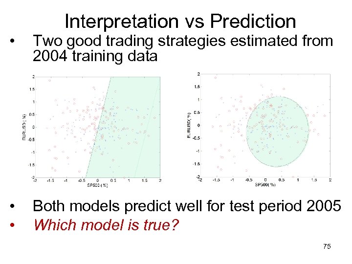Interpretation vs Prediction • Two good trading strategies estimated from 2004 training data • • Both models predict well for test period 2005 Which model is true? 75

Conclusions and Policy Implications • Market timing of international funds - has been indeed profitable in the past - does not work under present market conditions • Restrictions on frequent trading - reflect past market conditions - constrains risk management by small investors • Philosophical/policy question: can these trading restrictions be really justified? 76

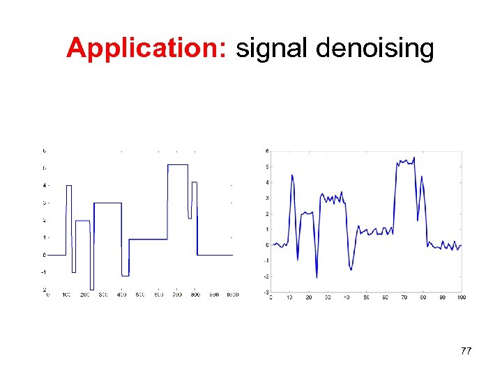Application: signal denoising 77

Signal denoising problem statement • Regression formulation ~ real-valued function estimation (with squared loss) • Signal representation: linear combination of orthogonal basis functions (harmonic, wavelets) • Differences (from standard formulation) - fixed sampling rate - training data x-values = test data x-values Computationally efficient orthogonal estimators: Discrete Fourier/Wavelet Transform (DFT / DWT) 78

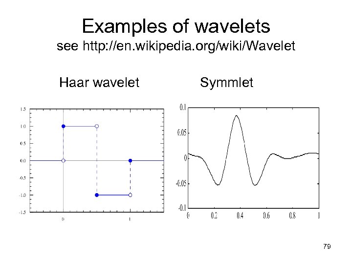Examples of wavelets see http: //en. wikipedia. org/wiki/Wavelet Haar wavelet Symmlet 79

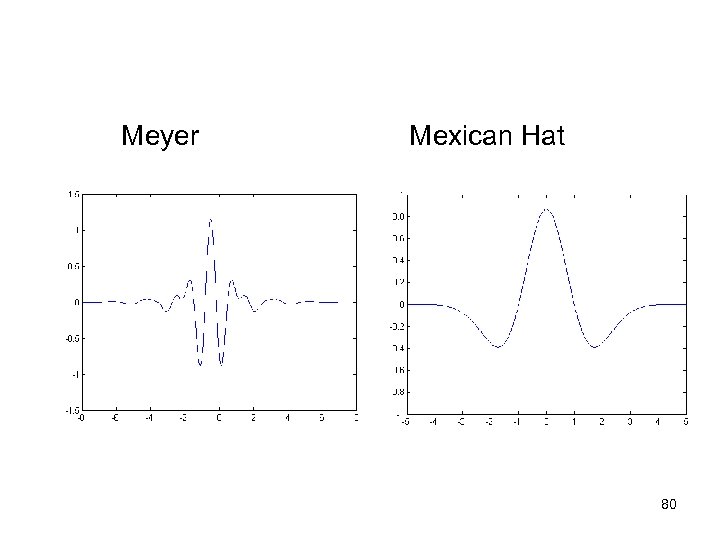Meyer Mexican Hat 80

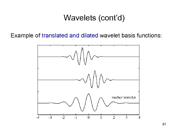Wavelets (cont’d) Example of translated and dilated wavelet basis functions: 81

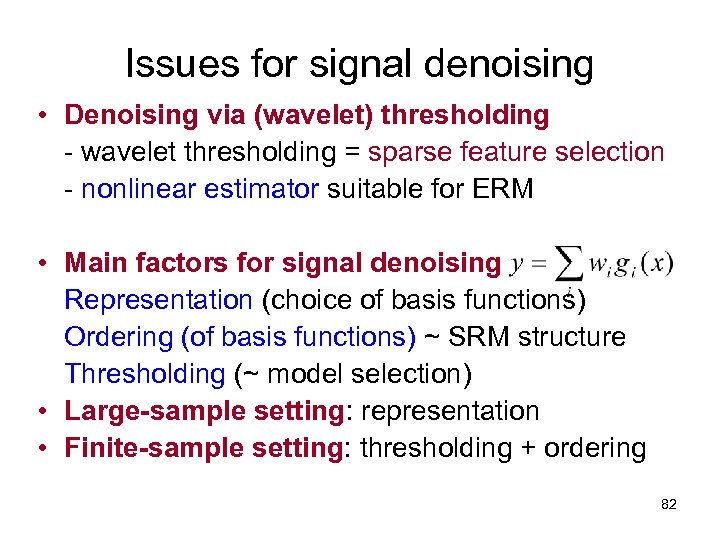Issues for signal denoising • Denoising via (wavelet) thresholding - wavelet thresholding = sparse feature selection - nonlinear estimator suitable for ERM • Main factors for signal denoising Representation (choice of basis functions) Ordering (of basis functions) ~ SRM structure Thresholding (~ model selection) • Large-sample setting: representation • Finite-sample setting: thresholding + ordering 82

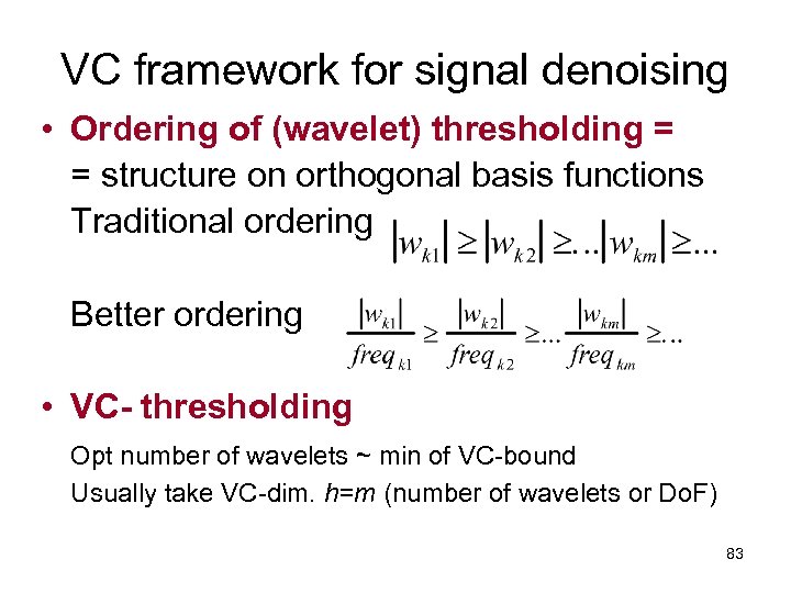VC framework for signal denoising • Ordering of (wavelet) thresholding = = structure on orthogonal basis functions Traditional ordering Better ordering • VC- thresholding Opt number of wavelets ~ min of VC-bound Usually take VC-dim. h=m (number of wavelets or Do. F) 83

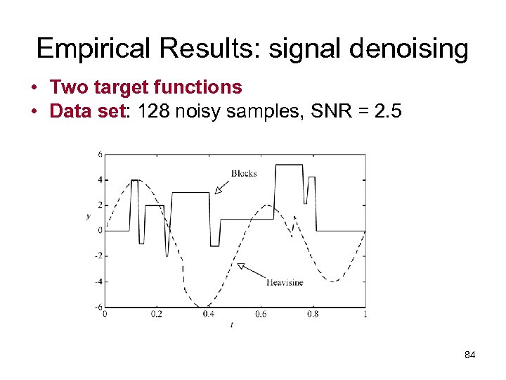Empirical Results: signal denoising • Two target functions • Data set: 128 noisy samples, SNR = 2. 5 84

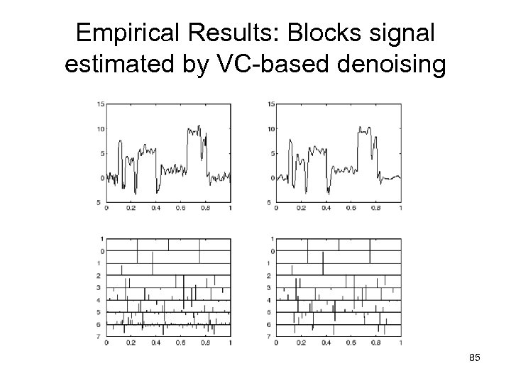Empirical Results: Blocks signal estimated by VC-based denoising 85

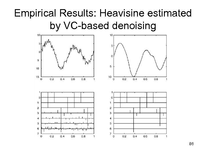Empirical Results: Heavisine estimated by VC-based denoising 86

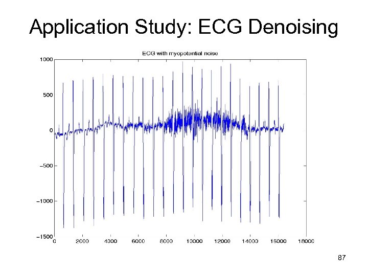Application Study: ECG Denoising 87

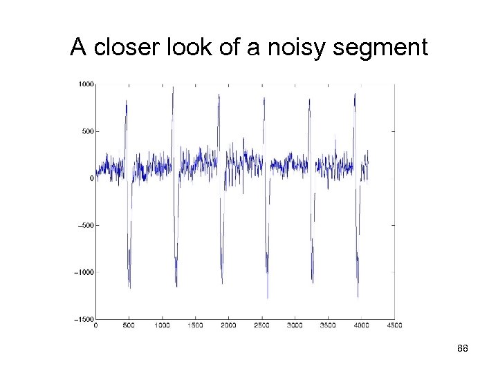A closer look of a noisy segment 88

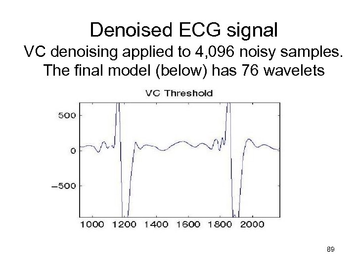Denoised ECG signal VC denoising applied to 4, 096 noisy samples. The final model (below) has 76 wavelets 89

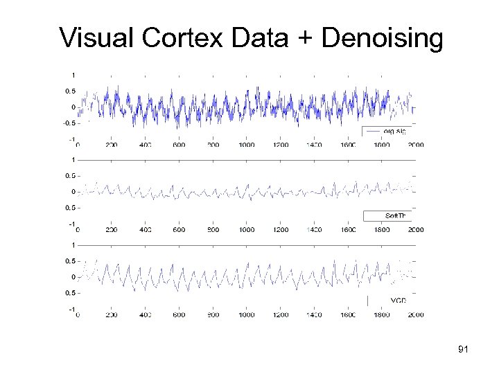
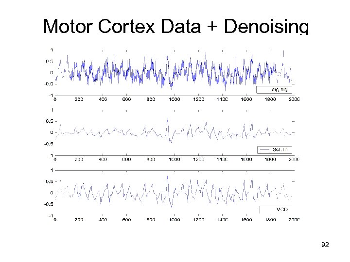
Application: f. MRI signal denoising • MOTIVATION: understanding brain function via functional MRI • DATA SET: provided by CMRR at UMN • Signals (~ waveforms) recorded at a certain brain location response to external stimulus applied 32 times • Data Set 1 ~ signals at the visual cortex in response to visual input light blinking 32 times • Data Set 2 ~ signals at the motor cortex recorded when human subject moves his finger 32 times • FMRI denoising = obtaining a better version of noisy signal 90

Visual Cortex Data + Denoising 91

Motor Cortex Data + Denoising 92

Discussion • Application of VC-theory to signal denoising - orthogonal basis functions - nonlinear estimator: sparse feature selection • Finite sample setting: importance of - Ordering (of basis functions) ~ SRM structure - Model selection (thresholding) • Large-sample setting: - type of basis functions (representation) 93

OUTLINE • Objectives • Inductive learning problem setting • Statistical Learning Theory • Applications • Measuring the VC-dimension • Summary and discussion 94

Measuring the VC-Dimension • • • VC-dimension is difficult to estimate (for most practical learning methods) Experimental estimation (Vapnik et al 1994) for binary classification problems Main idea: - apply learning method to randomly labeled data and measure the training error - the deviation of the training error from 0. 5 depends on the flexibility (VC-dimension) of an estimator. 95

Measuring the VC-Dimension • Experimental estimation (Vapnik et al 1994) for binary classification problems: - Based on theoretic analysis of the maximum deviation of error rates between two independently labeled data sets - Perform repeated random experiments with different data sets and sample sizes - Estimate VC-dim by fitting theoretic function (which depends only on n/h) 96

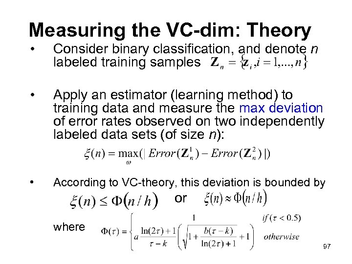Measuring the VC-dim: Theory • Consider binary classification, and denote n labeled training samples • Apply an estimator (learning method) to training data and measure the max deviation of error rates observed on two independently labeled data sets (of size n): • According to VC-theory, this deviation is bounded by or where 97

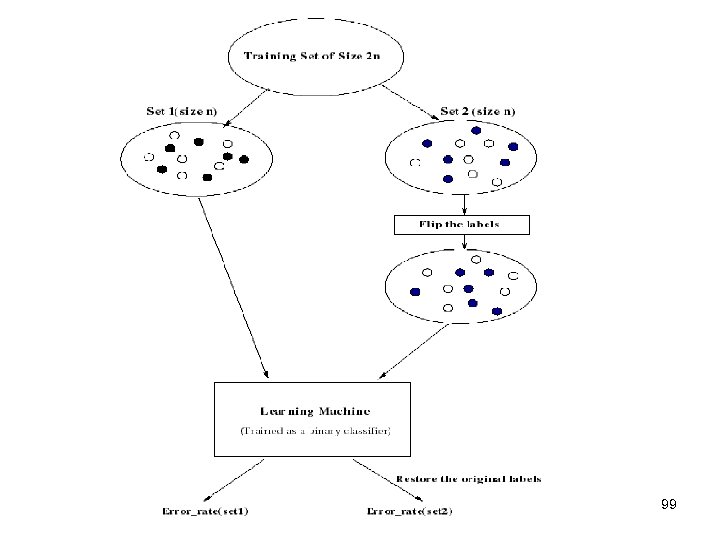
Measuring the VC-Dimension Using experimental measurements of we can fit these measurements to analytic function that depends only on VC-dim. Experimental procedure (for one measurement) - Generate a randomly labeled set of size 2 n - Split it into two sets of equal size: Z 1 and Z 2 - Flip the class labels for the second set Z 2 - Merge the two sets and train binary classifier - Separate the sets and flip the labels on the second set back again - Measure the difference between the error rates on the two sets: (n) = |Error(Z 1)-Error(Z 2)|. 98

99

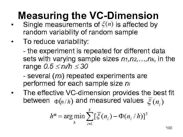• • • Measuring the VC-Dimension Single measurements of is affected by random variability of random sample To reduce variability: - the experiment is repeated for different data sets with varying sample sizes n 1, n 2, …, nk, in the range 0. 5 ni/h 30 - several (mi) repeated experiments are performed for each sample size ni The effective VC-dimension provides the best fit between and measured values 100

Measuring the VC-Dimension • Can be applied to estimating the VC-dimension of penalized estimators (ridge regression), i. e. finding dependency h=h(lambda) - see Example 7. 1 on p. 266 (in the textbook) • This dependency can be then used for analytic model selection using practical VC-bound Empirical results show that estimated VCdimension works better than using ‘effective’ Do. F for ridge regression, in conjunction with analytic model selection criteria. • 101

OUTLINE • Objectives • Inductive learning problem setting • Statistical Learning Theory • Applications • Measuring the VC-dimension • Summary and discussion 102

Summary and Discussion: VC-theory • Methodology - learning problem setting (KID principle) - concepts (risk minimization, VC-dim. , structure) • Interpretation/ evaluation of existing methods • Model selection using VC-bounds • Basis for new types of inference (TBD later) • Clear limitations/constraints for all learning methods based on the idea of ERM • What a theory cannot do: - provide formalization (for a given application) - select ‘good’ structure (for a given application) - always a gap between theory and applications 103

References • General references on VC-theory V. Vapnik, The Nature of Statistical Learning Theory, Springer, 1995 V. Vapnik, Statistical Learning Theory, Wiley, 1998 • Model selection using VC-bounds V. Cherkassky, X. Shao, F. Mulier and V. Vapnik, Model Complexity Control for regression using VC generalization bounds, IEEE Trans. on Neural Networks, 10, 5, 1075 -1089, 1999 V. Cherkassky and Y. Ma, Comparison of model selection for regression, Neural Computation, MIT Press 15 (7), 1691 -1714, 2003 • Market timing of international mutual funds V. Cherkassky and S. Dhar, Market Timing of International Funds: A Decade after the Scandal, Proc CIFEr 2012 • Measuring the VC-dimension V. Vapnik, E. Levin and Y Le Cun, Measuring the VC-dimension of a learning machine, Neural Computation, 6, 851 -876, 1994 X. Shao, V. Cherkassky and W. Li, Measuring the VC-dimension using optimized experimental design, Neural Computation, 12, 1969 -1986, 2000 • Signal denoising using VC-theory V. Cherkassky and X. Shao, Signal estimation and denoising using VC-theory, Neural Networks, Pergamon, 14, 37 -52, 2001 V. Cherkassky and S. Kilts, Myopotential denoising of ECG signals using wavelet thresholding methods, Neural Networks, Pergamon, 14, 1129 -1137, 2001 104