71a2530a72d62c041a0c2009c986cb8c.ppt
- Количество слайдов: 33
 Practical Process Control Using Control Station Prof. Doug Cooper Chemical Engineering Dept. University of Connecticut (Storrs) Copyright © 2002 Douglas J. Cooper All Rights Reserved
 1. Fundamental Principles of Process Control Motivation for Automatic Process Control n Safety First: – people, environment, equipment n The Profit Motive: – meeting final product specs – minimizing waste production – minimizing environmental impact – minimizing energy use – maximizing overall production rate Copyright © 2002 Douglas J. Cooper All Rights Reserved
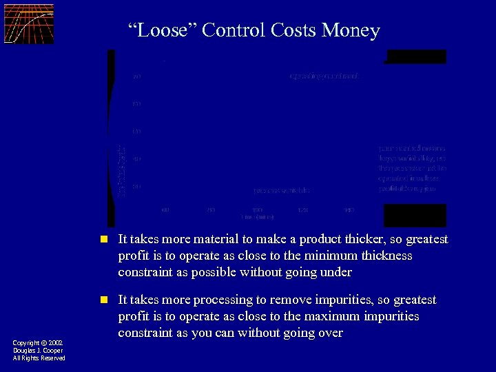 “Loose” Control Costs Money n n Copyright © 2002 Douglas J. Cooper All Rights Reserved It takes more material to make a product thicker, so greatest profit is to operate as close to the minimum thickness constraint as possible without going under It takes more processing to remove impurities, so greatest profit is to operate as close to the maximum impurities constraint as you can without going over
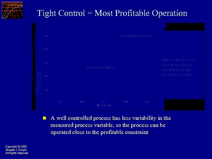 Tight Control = Most Profitable Operation n Copyright © 2002 Douglas J. Cooper All Rights Reserved A well controlled process has less variability in the measured process variable, so the process can be operated close to the profitable constraint
 An introductory example Copyright © 2002 Douglas J. Cooper All Rights Reserved
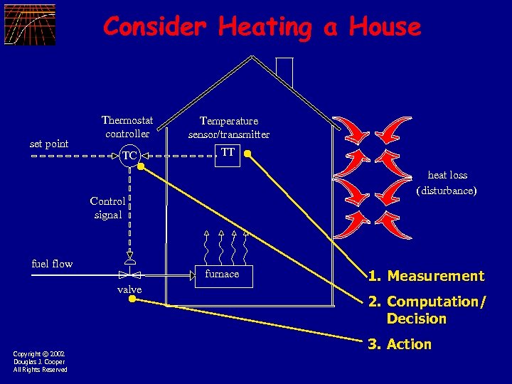 Consider Heating a House set point Thermostat controller Temperature sensor/transmitter TC TT heat loss (disturbance) Control signal fuel flow furnace valve Copyright © 2002 Douglas J. Cooper All Rights Reserved 1. Measurement 2. Computation/ Decision 3. Action
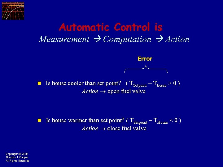 Automatic Control is Measurement Computation Action Error n Is house cooler than set point? ( TSetpoint Thouse > 0 ) Action open fuel valve n Is house warmer than set point? ( TSetpoint THouse < 0 ) Action close fuel valve Copyright © 2002 Douglas J. Cooper All Rights Reserved
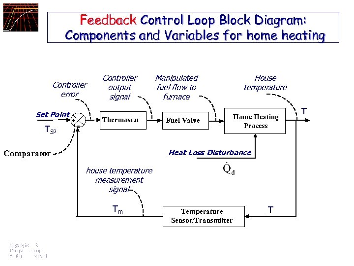 Feedback Control Loop Block Diagram: Components and Variables for home heating Controller error Set Point TSP + - Controller output signal Thermostat Manipulated fuel flow to furnace Fuel Valve House temperature Home Heating Process Heat Loss Disturbance Comparator house temperature measurement signal Tm Copyright © 2002 Douglas J. Cooper All Rights Reserved Temperature Sensor/Transmitter T T
 Terminology Control Objective Copyright © 2002 Douglas J. Cooper All Rights Reserved Controlled Process Variable Measured Variable Set point Error Controller Output Manipulated Variable Disturbances
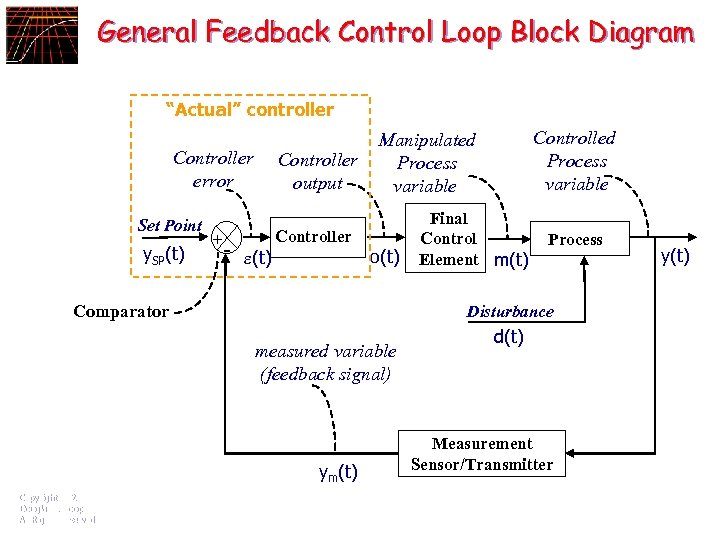 General Feedback Control Loop Block Diagram “Actual” controller Controller error Set Point y. SP(t) + Controller output - (t) Controller o(t) Comparator Final Control Element m(t) Process Disturbance measured variable (feedback signal) ym(t) Copyright © 2002 Douglas J. Cooper All Rights Reserved Controlled Process variable Manipulated Process variable d(t) Measurement Sensor/Transmitter y(t)
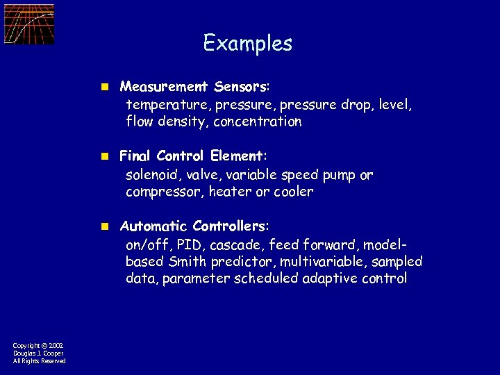 Examples n n Final Control Element: solenoid, valve, variable speed pump or compressor, heater or cooler n Copyright © 2002 Douglas J. Cooper All Rights Reserved Measurement Sensors: temperature, pressure drop, level, flow density, concentration Automatic Controllers: on/off, PID, cascade, feed forward, modelbased Smith predictor, multivariable, sampled data, parameter scheduled adaptive control
 3. Graphical Modeling of Dynamic Process Data Process Behavior and Controller Tuning n Consider cruise control for a car vs a truck – how quickly can each accelerate or decelerate – what is the effect of disturbances (wind, hills, etc. ) n Controller (gas flow) manipulations required to maintain set point velocity in spite of disturbances (wind, hills) are different for a car and truck because the dynamic behavior of each "process" is different Dynamic behavior how the measured process variable responds over time to changes in the controller output and disturbance variables Copyright © 2002 Douglas J. Cooper All Rights Reserved
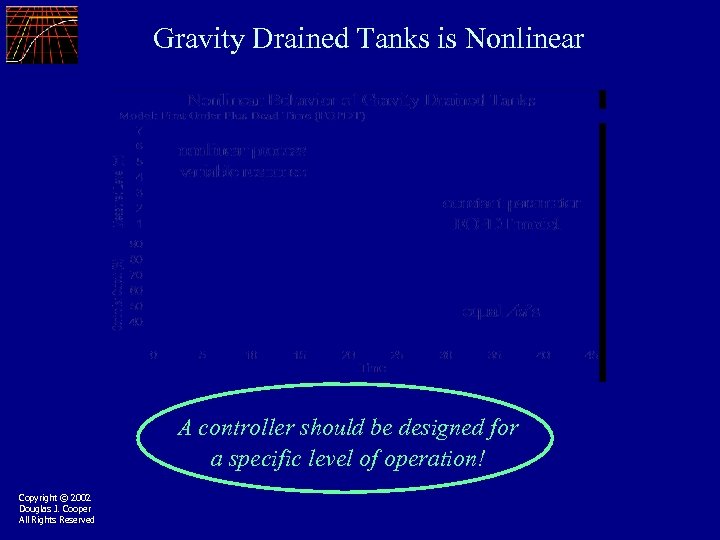
 Understanding Dynamic Process Behavior n n Process variable test data can be generated by suddenly changing the controller output signal n Be sure to move the controller output far enough and fast enough so that the dynamic behavior of the process is clearly revealed as the process responds n Copyright © 2002 Douglas J. Cooper All Rights Reserved To learn about the dynamic behavior of a process, analyze measured process variable test data The dynamic behavior of a process is different as operating level changes (nonlinear behavior) so collect process data at normal operating levels (design level of operation)
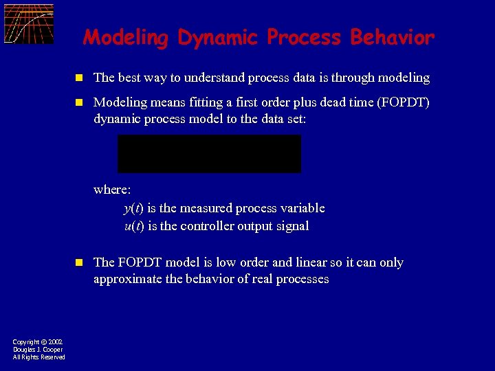 Modeling Dynamic Process Behavior n The best way to understand process data is through modeling n Modeling means fitting a first order plus dead time (FOPDT) dynamic process model to the data set: where: y(t) is the measured process variable u(t) is the controller output signal n Copyright © 2002 Douglas J. Cooper All Rights Reserved The FOPDT model is low order and linear so it can only approximate the behavior of real processes
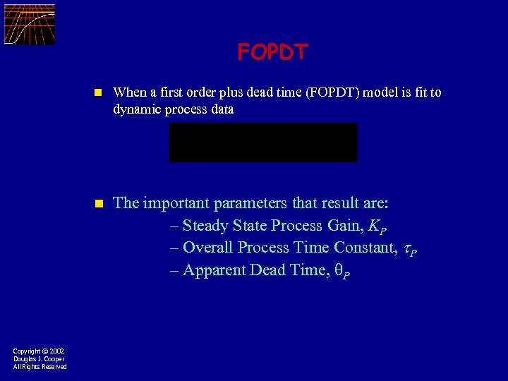 FOPDT n When a first order plus dead time (FOPDT) model is fit to dynamic process data n Copyright © 2002 Douglas J. Cooper All Rights Reserved The important parameters that result are: – Steady State Process Gain, KP – Overall Process Time Constant, P – Apparent Dead Time, P
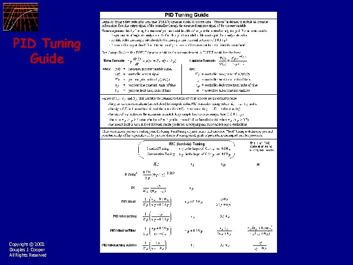 PID Tuning Guide Copyright © 2002 Douglas J. Cooper All Rights Reserved
 The FOPDT Model is All Important n n sign of KP indicates the action of the controller (+KP reverse acting; KP direct acting) n size of P indicates the maximum desirable loop sample time (be sure sample time T 0. 1 P) n ratio P / P indicates whether MPC (Smith predictor) would show benefit (useful if P P) n Copyright © 2002 Douglas J. Cooper All Rights Reserved model parameters (KP, P and P) are used in correlations to compute initial controller tuning values model becomes part of the feed forward, Smith predictor, decoupling and other model-based controllers
 Step Test Copyright © 2002 Douglas J. Cooper All Rights Reserved n n The controller is set to manual mode Process starts at steady state Controller output signal is stepped to new value Measured process variable allowed to complete response
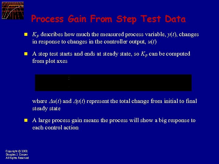 Process Gain From Step Test Data n KP describes how much the measured process variable, y(t), changes in response to changes in the controller output, u(t) n A step test starts and ends at steady state, so KP can be computed from plot axes where u(t) and y(t) represent the total change from initial to final steady state n Copyright © 2002 Douglas J. Cooper All Rights Reserved A large process gain means the process will show a big response to each control action
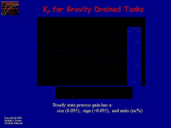 KP for Gravity Drained Tanks Steady state process gain has a: size (0. 095), sign (+0. 095), and units (m/%) Copyright © 2002 Douglas J. Cooper All Rights Reserved
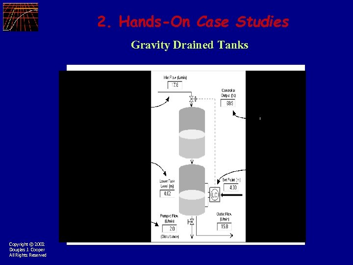 2. Hands-On Case Studies Gravity Drained Tanks Copyright © 2002 Douglas J. Cooper All Rights Reserved
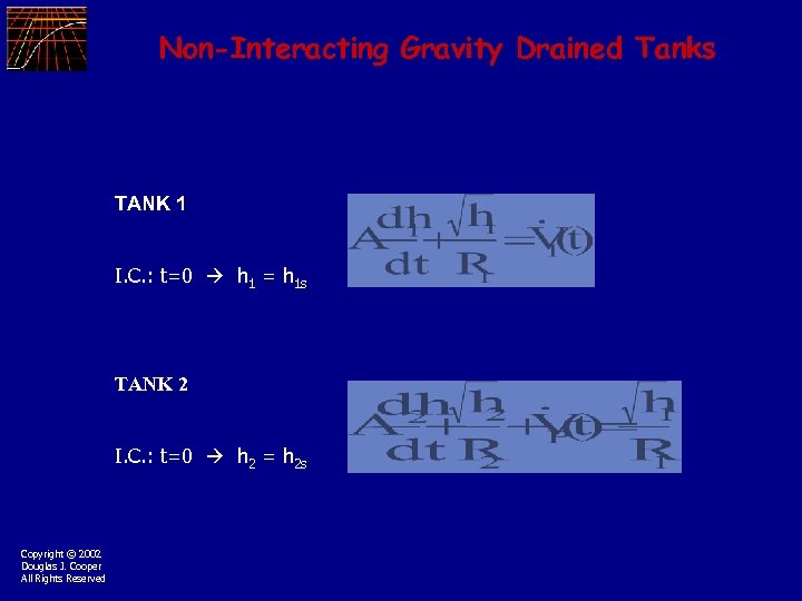 Non-Interacting Gravity Drained Tanks TANK 1 I. C. : t=0 h 1 = h 1 s TANK 2 I. C. : t=0 h 2 = h 2 s Copyright © 2002 Douglas J. Cooper All Rights Reserved
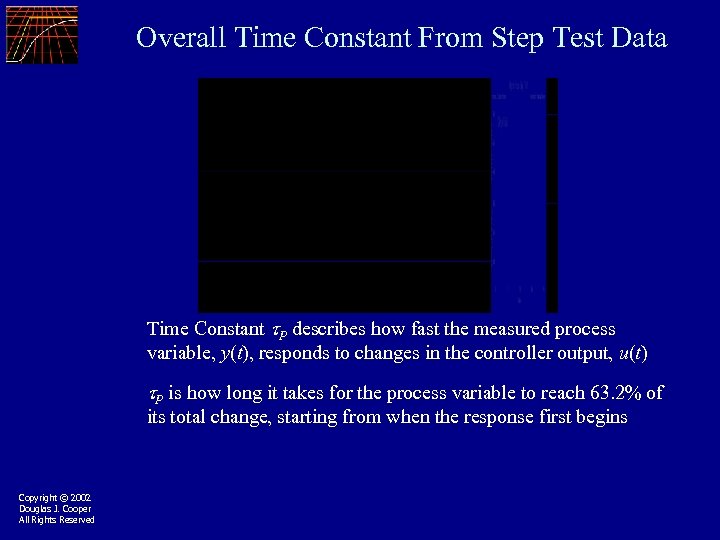 Overall Time Constant From Step Test Data Time Constant P describes how fast the measured process variable, y(t), responds to changes in the controller output, u(t) P is how long it takes for the process variable to reach 63. 2% of its total change, starting from when the response first begins Copyright © 2002 Douglas J. Cooper All Rights Reserved
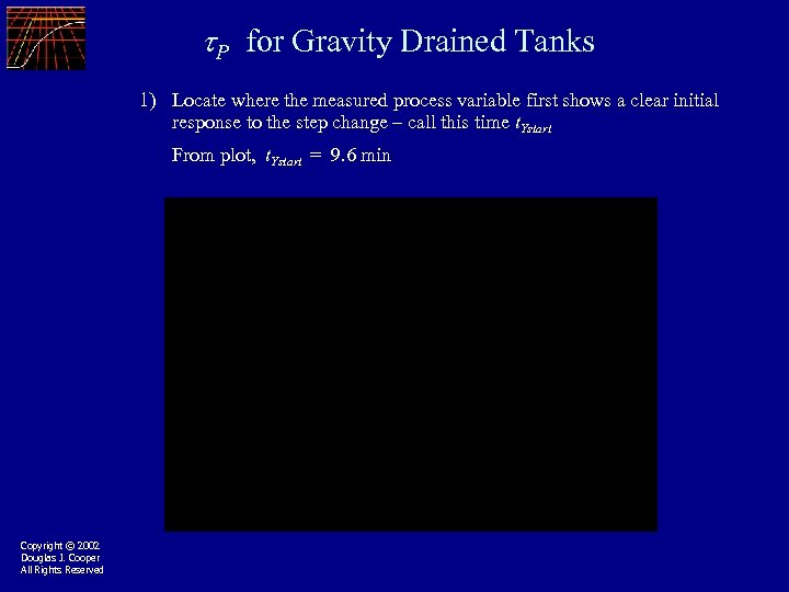 P for Gravity Drained Tanks 1) Locate where the measured process variable first shows a clear initial response to the step change – call this time t. Ystart From plot, t. Ystart = 9. 6 min Copyright © 2002 Douglas J. Cooper All Rights Reserved
 P for Gravity Drained Tanks 2) Locate where the measured process variable reaches y 63. 2, or where y(t) reaches 63. 2% of its total final change Label time t 63. 2 as the point in time where y 63. 2 occurs Copyright © 2002 Douglas J. Cooper All Rights Reserved
 P for Gravity Drained Tanks n n y 63. 2 = 1. 93 m + 0. 632( y) = 1. 93 m + 0. 632(0. 95 m) = 2. 53 m n Copyright © 2002 Douglas J. Cooper All Rights Reserved y(t) starts at 1. 93 m and shows a total change y = 0. 95 m y(t) passes through 2. 53 m at t 63. 2 = 11. 2 min
 P for Gravity Drained Tanks - The time constant is the time difference between t. Ystart and t 63. 2 - Time constant must be positive and have units of time From the plot: P = t 63. 2 t. Ystart = 11. 2 min 9. 6 min = 1. 6 min Copyright © 2002 Douglas J. Cooper All Rights Reserved
 Apparent Dead Time From Step Test Data n P is the time from when the controller output step is made until when the measured process variable first responds n Apparent dead time, P, is the sum of these effects: – transportation lag, or the time it takes for material to travel from one point to another – sample or instrument lag, or the time it takes to collect analyze or process a measured variable sample – higher order processes naturally appear slow to respond n Copyright © 2002 Douglas J. Cooper All Rights Reserved Notes: – Dead time must be positive and have units of time – Tight control in increasingly difficult as P 0. 7 P – For important loops, work to avoid unnecessary dead time
 P for Gravity Drained Tanks P = t. Ystart t. Ustep = 9. 6 min 9. 2 min = 0. 4 min Copyright © 2002 Douglas J. Cooper All Rights Reserved
 Workshop 1: Exploring Dynamics of Gravity Drained Tanks Copyright © 2002 Douglas J. Cooper All Rights Reserved
 Processes Have Time-Varying Behaviors n n But real processes change every day because – surfaces foul or corrode – mechanical elements like seals or bearings wear – feedstock quality varies and catalyst activity drifts – environmental conditions like heat and humidity change n So the values of KP, P that best describe the dynamic behavior of a process today may not be best tomorrow n Copyright © 2002 Douglas J. Cooper All Rights Reserved The predictions of a FOPDT model are constant over time As a result, controller performance will degrade with time and periodic retuning may be required
 Processes Have Nonlinear Behaviors The predictions of a FOPDT model are constant as operating level changes n The response of a real process varies with operating level n Copyright © 2002 Douglas J. Cooper All Rights Reserved
 Gravity Drained Tanks is Nonlinear A controller should be designed for a specific level of operation! Copyright © 2002 Douglas J. Cooper All Rights Reserved


