lecture_3.pptx
- Количество слайдов: 22
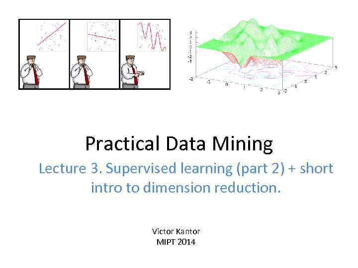 Practical Data Mining Lecture 3. Supervised learning (part 2) + short intro to dimension reduction. Victor Kantor MIPT 2014
 Plan 1. Bayesian methods 2. Linear methods introduction 3. Principal component and SVD introduction 4. Python, scikit-learn and kaggle. com
 Bayesian methods 1. Spam classification with Naïve Bayes classifier 2. Probabilities estimation 3. Loss function and risk function
 Intro: simple idea of spam detection Spam message examples: • “Hi! : ) Purchase Exclusive Tabs Online http: //. . . ” • “We Offer Loan At A Very Low Rate Of 3%. If Interested, Kindly Contact Us, Reply by this email …. @hotmail. com”
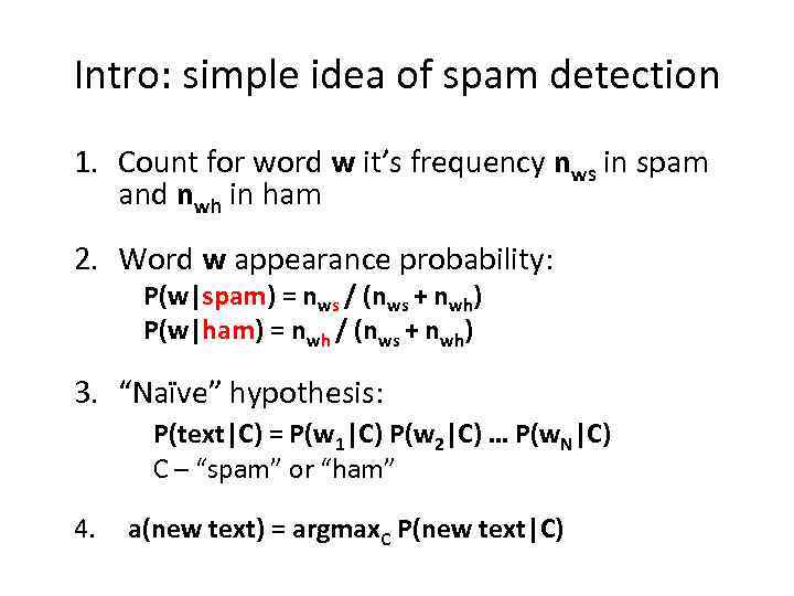 Intro: simple idea of spam detection 1. Count for word w it’s frequency nws in spam and nwh in ham 2. Word w appearance probability: P(w|spam) = nws / (nws + nwh) P(w|ham) = nwh / (nws + nwh) 3. “Naïve” hypothesis: P(text|C) = P(w 1|C) P(w 2|C) … P(w. N|C) C – “spam” or “ham” 4. a(new text) = argmax. C P(new text|C)
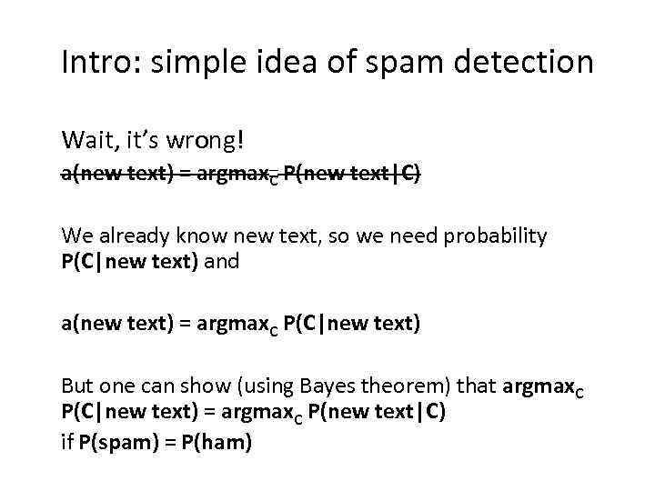 Intro: simple idea of spam detection Wait, it’s wrong! a(new text) = argmax. C P(new text|C) We already know new text, so we need probability P(C|new text) and a(new text) = argmax. C P(C|new text) But one can show (using Bayes theorem) that argmax. C P(C|new text) = argmax. C P(new text|C) if P(spam) = P(ham)
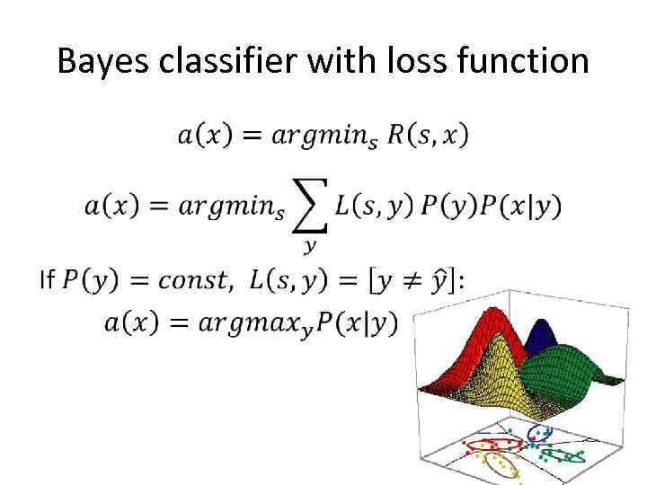
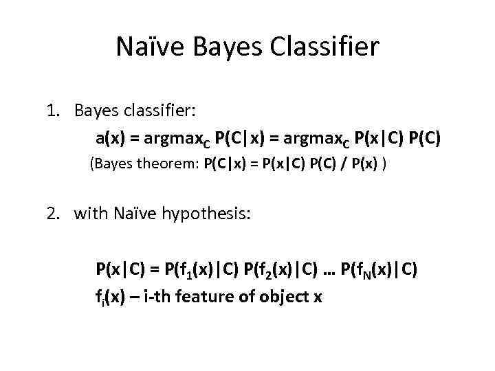 Naïve Bayes Classifier 1. Bayes classifier: a(x) = argmax. C P(C|x) = argmax. C P(x|C) P(C) (Bayes theorem: P(C|x) = P(x|C) P(C) / P(x) ) 2. with Naïve hypothesis: P(x|C) = P(f 1(x)|C) P(f 2(x)|C) … P(f. N(x)|C) fi(x) – i-th feature of object x
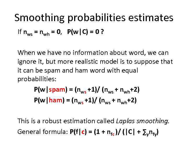 Smoothing probabilities estimates If nws = nwh = 0, P(w|C) = 0 ? When we have no information about word, we can ignore it, but more realistic model is to suppose that it can be spam and ham word with equal probabilities: P(w|spam) = (nws +1)/ (nws + nwh+2) P(w|ham) = (nws +1)/ (nws + nwh+2) This is a robust estimation called Laplas smoothing. General formula: P(f|c) = (1 + nfc )/ (|C| + ∑ynfy)
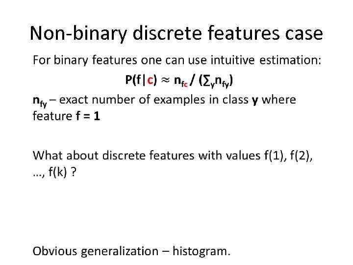 Non-binary discrete features case •
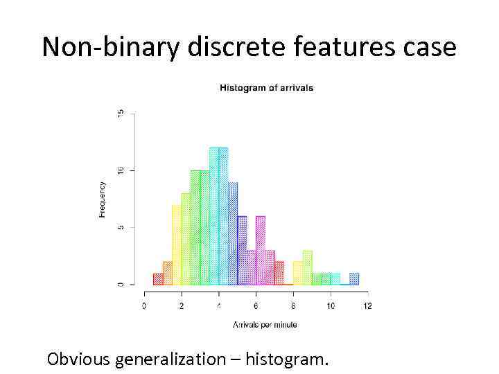 Non-binary discrete features case Obvious generalization – histogram.
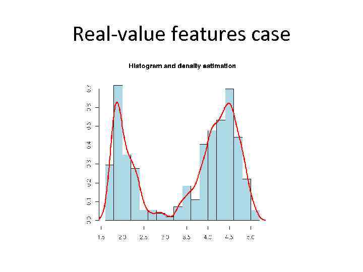
 Real-value features case X: What about real-value features? Y: Make it discrete! Z: And smooth!
 Real-value features case
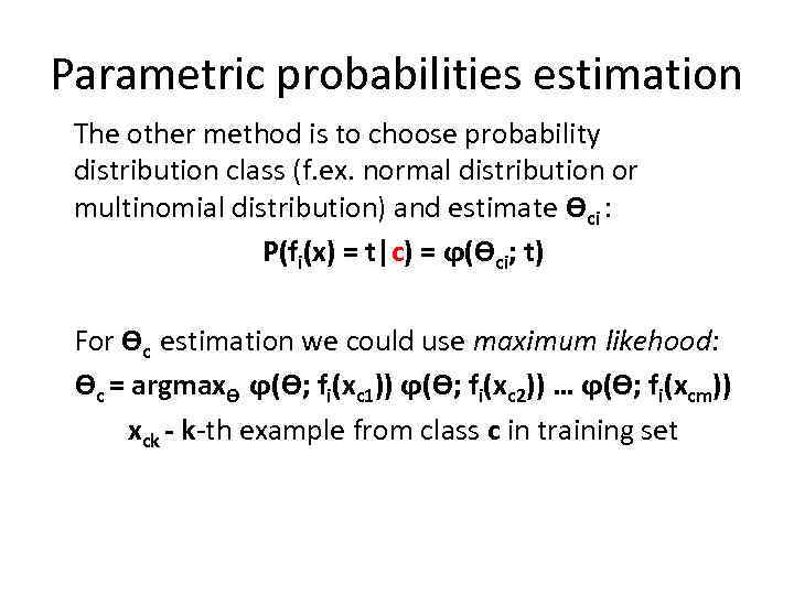 Parametric probabilities estimation The other method is to choose probability distribution class (f. ex. normal distribution or multinomial distribution) and estimate ϴci : P(fi(x) = t|c) = ϕ(ϴci; t) For ϴc estimation we could use maximum likehood: ϴc = argmaxϴ ϕ(ϴ; fi(xc 1)) ϕ(ϴ; fi(xc 2)) … ϕ(ϴ; fi(xcm)) xck - k-th example from class c in training set
 Distribution class choice recommendations • Text features/other sparse discrete features – multinomial distribution • Continuous features with low scatter – normal distribution • Continuous features with outliers – distributions with “heavy tail”
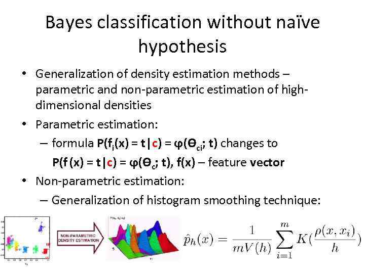 Bayes classification without naïve hypothesis • Generalization of density estimation methods – parametric and non-parametric estimation of highdimensional densities • Parametric estimation: – formula P(fi(x) = t|c) = ϕ(ϴci; t) changes to P(f (x) = t|c) = ϕ(ϴc; t), f(x) – feature vector • Non-parametric estimation: – Generalization of histogram smoothing technique:
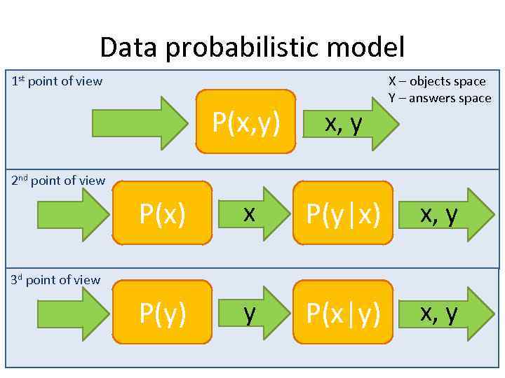 Data probabilistic model 1 st point of view X – objects space Y – answers space P(x, y) x, y P(x) x P(y|x) x, y P(y) y P(x|y) x, y 2 nd point of view 3 d point of view
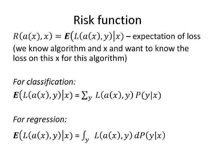
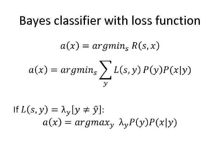
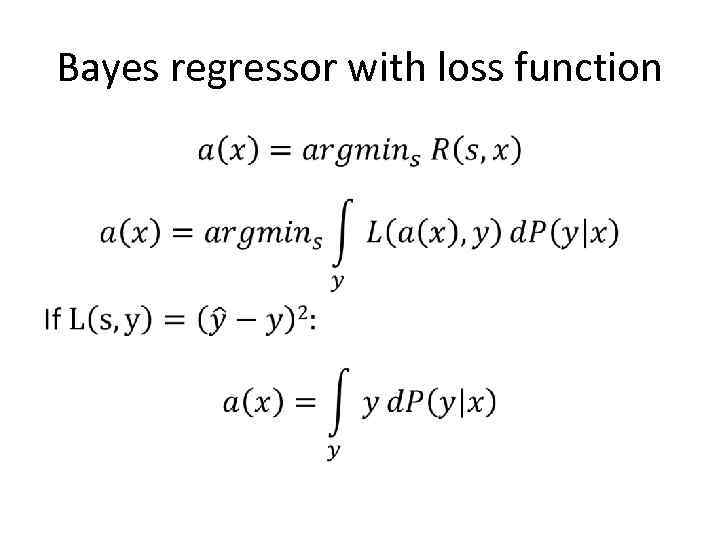
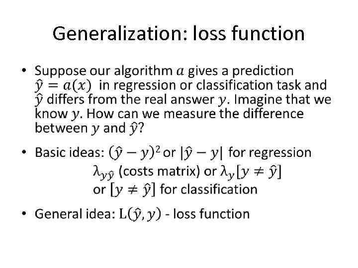 Generalization: loss function •
 Risk function •
 Bayes classifier with loss function •
 Bayes classifier with loss function •
 Bayes regressor with loss function •
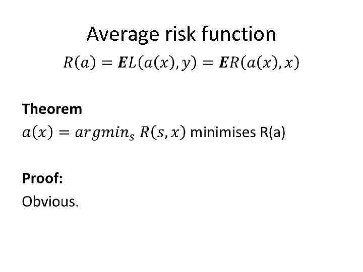 Average risk function •


