12860080d34296367d268b7d09be0700.ppt
- Количество слайдов: 100
Poverty and Inequality Course, World Bank, March 2008 Poverty, Inequality and Growth: Debates, Concepts and Evidence Martin Ravallion Development Research Group, World Bank
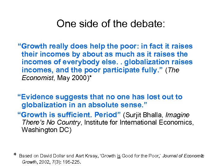
One side of the debate: “Growth really does help the poor: in fact it raises their incomes by about as much as it raises the incomes of everybody else. . globalization raises incomes, and the poor participate fully. ” (The Economist, May 2000)* “Evidence suggests that no one has lost out to globalization in an absolute sense. ” “Growth is sufficient. Period” (Surjit Bhalla, Imagine There’s No Country, Institute for International Economics, Washington DC) 2 * Based on David Dollar and Aart Kraay, ‘Growth is Good for the Poor, ’ Journal of Economic Growth, 2002, 7(3): 195 -225.
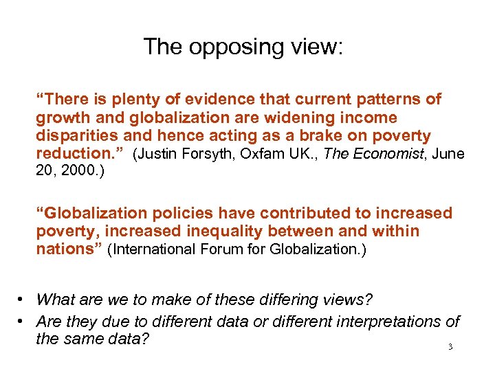
The opposing view: “There is plenty of evidence that current patterns of growth and globalization are widening income disparities and hence acting as a brake on poverty reduction. ” (Justin Forsyth, Oxfam UK. , The Economist, June 20, 2000. ) “Globalization policies have contributed to increased poverty, increased inequality between and within nations” (International Forum for Globalization. ) • What are we to make of these differing views? • Are they due to different data or different interpretations of the same data? 3
1 Concepts and measures 2 Evidence from cross-country comparisons 3 Evidence for China and India 4 Some implications for policy 4

1 Concepts and measures Confusion galore in the globalization debate “inequality” “pro-poor growth” 5
What do we mean by “inequality”? Two very different definitions in public debates and policy discussions 6
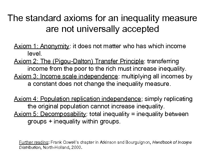
The standard axioms for an inequality measure are not universally accepted Axiom 1: Anonymity: it does not matter who has which income level. Axiom 2: The (Pigou-Dalton) Transfer Principle: transferring income from the poor to the rich must increase inequality. Axiom 3: Income scale independence: multiplying all incomes by a constant does not change the inequality measure. Axiom 4: Population replication independence; simply replicating the original population cannot increase inequality. Axiom 5: Decomposability: total inequality = inequality between groups + inequality within groups. Further reading: Frank Cowell’s chapter in Atkinson and Bourguignon, Handbook of Income 7 Distribution, North-Holland, 2000.
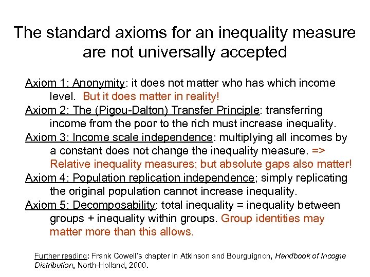
The standard axioms for an inequality measure are not universally accepted Axiom 1: Anonymity: it does not matter who has which income level. But it does matter in reality! Axiom 2: The (Pigou-Dalton) Transfer Principle: transferring income from the poor to the rich must increase inequality. Axiom 3: Income scale independence: multiplying all incomes by a constant does not change the inequality measure. => Relative inequality measures; but absolute gaps also matter! Axiom 4: Population replication independence; simply replicating the original population cannot increase inequality. Axiom 5: Decomposability: total inequality = inequality between groups + inequality within groups. Group identities may matter more than this allows. Further reading: Frank Cowell’s chapter in Atkinson and Bourguignon, Handbook of Income 8 Distribution, North-Holland, 2000.
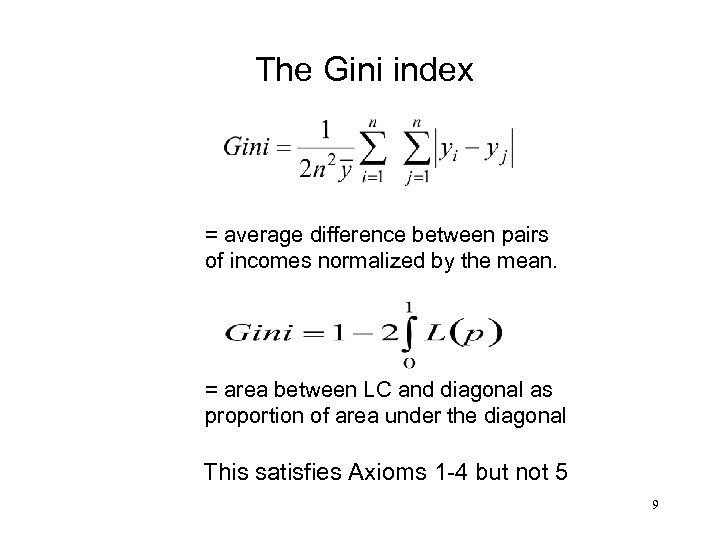
The Gini index = average difference between pairs of incomes normalized by the mean. = area between LC and diagonal as proportion of area under the diagonal This satisfies Axioms 1 -4 but not 5 9
Gini index graphically Gini index=A/(A+B) Area A Area B 10

What values does the Gini index take? • Bounded between zero (everyone has the mean income) and unity (the richest person has all the income) • What values do we find in practice? Gini index (country-level) ranges from about 0. 25 to 0. 65, which is also (roughly) the Gini index for the world as a whole. 11

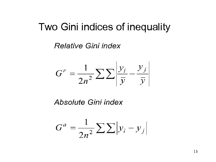
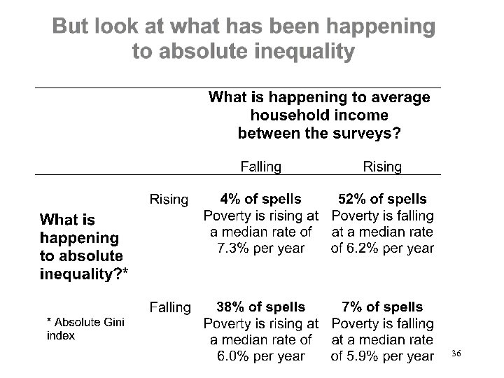
Relative vs. absolute inequality • Relative inequality is about ratios; absolute inequality is about differences. – State A: two incomes $1, 000 and $10, 000 per year – State B: these rise to $2, 000 and $20, 000 – Ratio is unchanged but the “rich” can buy 10 times more from the income gains in state B than can the “poor” • One is not right and the other wrong. Indeed, 40% of participants in experiments view inequality in absolute terms. • As we will see, whether one thinks about inequality as absolute or relative matters greatly to one’s views on the distribution of the gains from growth. Further reading: Amiel and Cowell, Thinking about Inequality, Cambridge: Cambridge University Press, 1999 12
Two Gini indices of inequality 13
What do we mean by “pro-poor growth”? Again, two very different definitions 14

Definition 1: Pro-poor growth= growth with pro-poor redistribution • Changes in distribution are poverty reducing, i. e. , poverty falls by more than one would have expected holding distribution constant (1). => A negative “redistribution component” in the Datt. Ravallion (2) decomposition for changes in poverty. • Let P(µ, L) = poverty measure with mean µ and a vector of parameters, L, describing the Lorenz curve. • The change in poverty between dates 1 and 2 (say) is “pro poor” if P(µr, L 2) < P(µr, L 1) for some fixed µr Further reading: 1. Nanak Kakwani and E. Pernia, (2000), ‘What Is Pro-Poor Growth? ’ Asian Development Review. 18(1): 1 -16. 2. Gaurav Datt and Martin Ravallion (1992), ‘Growth and Redistribution Components of Changes in Poverty Measures: A Decomposition with Applications to Brazil and India in the 1980 s’, Journal of Development Economics, 38, 275 -295. 15
However, … • By this definition, distributional changes can be “propoor” with no absolute gain to the poor, or even falling living standards for poor people. • Equally well, “pro-rich” distributional shifts may have come with large absolute gains to the poor. 16
Definition 2: Pro-poor growth= growth that benefits poor people Growth is pro-poor if and only if it accompanies a reduction in an agreed measure of poverty. * But what measure of poverty? * Martin Ravallion and Shaohua Chen, “Measuring Pro-Poor Growth”, Economics Letters, 2003. 17

The Watts Index… • is the mean proportionate poverty gap of the poor: where: the headcount index is Ht=Ft(z), z=poverty line; yt(p) is the quantile function (inverse of p=Ft(yt)). • This is the only index that satisfies all accepted axioms for poverty measurement including: focus axiom, monotonicity axiom; transfer axiom, transfersensitivity and subgroup consistency (2). Further reading: 1. Harold Watts, “An Economic Definition of Poverty, ” in D. P. Moynihan (ed. ), On Understanding Poverty. New York, Basic Books, 1968. 2. Buhong Zheng, “Axiomatic Characterization of the Watts Index, ” Economics Letters 1993, 42, 81 -86. 18

Growth incidence curve where yt(p) is the quantile function: yt=Ft-1(p) 19

A measure of pro-poor growth consistent with the Watts index The Ravallion-Chen measure of the “rate of propoor growth” is the mean growth rate of the poor: = area under the growth incidence curve up to H normalized by H. Further reading: Martin Ravallion and Shaohua Chen, “Measuring Pro-Poor Growth”, Economics Letters, 2003. 20
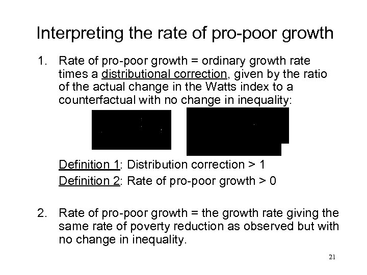
Interpreting the rate of pro-poor growth 1. Rate of pro-poor growth = ordinary growth rate times a distributional correction, given by the ratio of the actual change in the Watts index to a counterfactual with no change in inequality: Definition 1: Distribution correction > 1 Definition 2: Rate of pro-poor growth > 0 2. Rate of pro-poor growth = the growth rate giving the same rate of poverty reduction as observed but with no change in inequality. 21
Note: g. H is not the growth rate in the mean income of the poor … which does not satisfy either the monotonicity or transfer axioms. • If an initially poor person above the mean escapes poverty then the growth rate in the mean for the poor will be negative; yet poverty has fallen. • This problem is avoided if one fixes H; • but then the measure fails the focus and transfer axioms. 22
2 Evidence from cross-country comparisons Does growth come with rising inequality? Does growth reduce poverty? 23
The Kuznets Hypothesis • Relative inequality increases in the early stages of growth in a developing country but begins to fall after some point, • i. e. , the relationship between inequality (on the vertical axis) and average income (horizontal) is predicted to trace out an inverted U. Further reading: Sudhir Anand Ravi Kanbur, “The Kuznets Process and the Inequality. Development Relationship, ” Journal of Development Economics 1993, Vol. 40: 25 -52. 24

Why might the KH hold? • Assume that the economy comprises: – a low-inequality and poor (low-mean) rural sector, and – a richer urban sector with higher inequality. • Growth occurs by rural labor shifting to the urban sector. • Assume that the migration process is such that a representative slice of the rural distribution is transformed into a representative slice of the urban distribution. – i. e. , distribution is unchanged within each sector. • Starting with all the population in the rural sector, when the first worker moves to the urban sector, inequality must increase even though the incidence of poverty has fallen. • And when the last rural worker leaves, inequality falls. • Between these extremes, there will be a turning point. 25
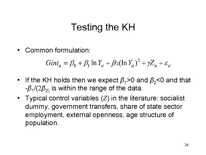
Testing the KH • Common formulation: • If the KH holds then we expect β 1>0 and β 2<0 and that -β 1/(2β 2) is within the range of the data. • Typical control variables (Z) in the literature: socialist dummy, government transfers, share of state sector employment, external openness, age structure of population. 26
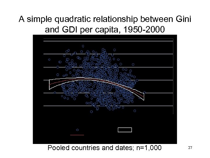
A simple quadratic relationship between Gini and GDI per capita, 1950 -2000 Pooled countries and dates; n=1, 000 27

• A weak inverted U relationship (more than 1000 Ginis) • Huge variability in inequality; R 2 only 0. 08 • The upward sloping part of the curve particularly hard to discern • Turning point is quite unstable; here about $PPP 2, 000 (level of Senegal or Zimbabwe) • Even this weak inverted U vanishes with country fixed effects. The most serious critique: With greater time series evidence, we find that very few developing countries have followed the prediction of KH. * Further reading: * Bruno, Michael, Martin Ravallion and Lyn Squire (1998), “Equity and Growth in Developing Countries: Old and New Perspectives on the Policy Issues, ” in Income Distribution and High-Quality Growth (edited by Vito Tanzi and Ke-young Chu), Cambridge, Mass: MITPress. 28
Changes in relative inequality are uncorrelated with growth 1. Across 120 spells (between two surveys), virtually zero correlation between changes in inequality (the log Gini index) and economic growth (change in the log of the survey mean or PCE). * Figure=> 2. Mean income of the poorest 20% (say) has a regression coefficient of about one on the overall growth rate** Further reading: * Martin Ravallion, “Inequality is Bad for the Poor, ” in Inequality and Poverty Re-Examined, edited by John Micklewright and Steven Jenkins, Oxford: Oxford University Press, forthcoming. **David Dollar and Aart Kraay, ‘Growth is Good for the Poor, ’ Journal of Economic Growth, 2002, 29 7(3): 195 -225.

r = – 0. 13 30
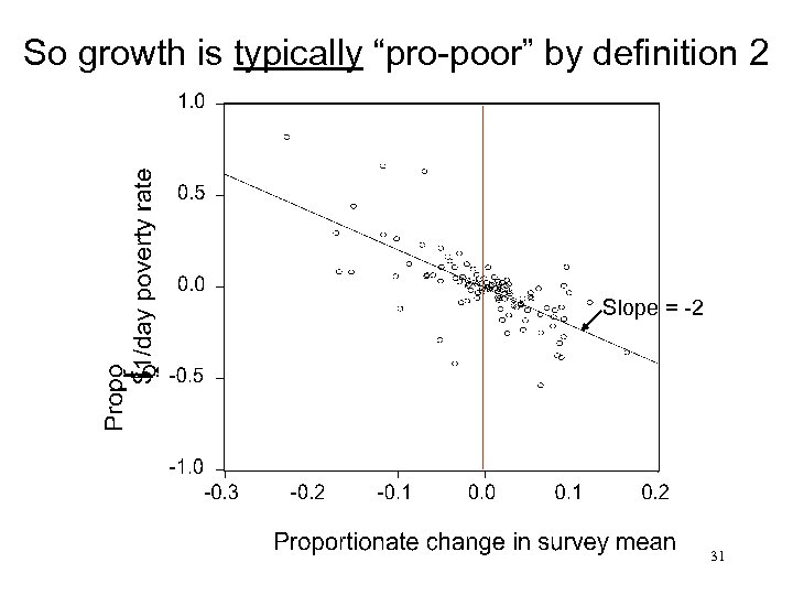
So growth is typically “pro-poor” by definition 2 Slope = -2 31

The extent to which growth is pro-poor has varied enormously between countries and over time • A 1% rate of growth will bring anything from a modest drop in the poverty rate of 0. 6% to a more dramatic 3. 5% annual decline (95% CI). • There have been plenty of cases of rising inequality during spells of growth. Indeed, inequality increases about half the time Further reading: Martin Ravallion, “Growth, Inequality and Poverty: Looking Beyond Averages, ” 32 World Development, Vol. 29(11), November 2001, pp. 1803 -1815.
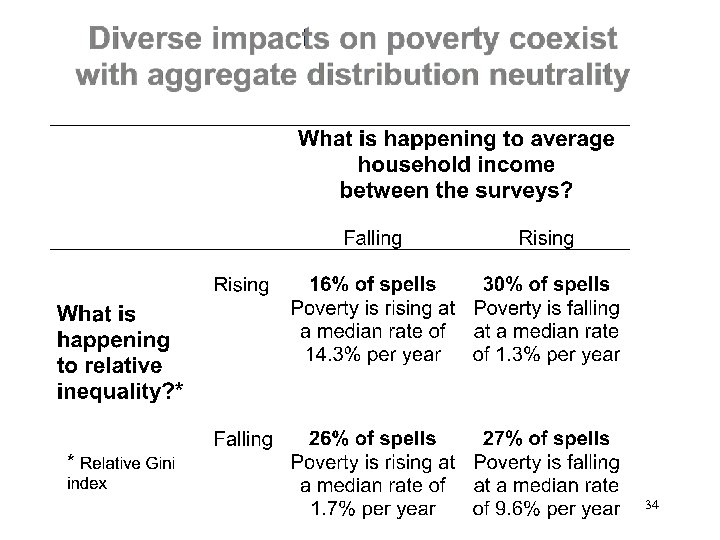
Distribution-neutrality on average does not mean that distribution is unchanging; in fact, it changes a lot • Large fluctuations in measured inequality even when no long-run trend • Some of this is measurement error; noise in inequality data • But even seemingly small changes in a Gini index (say) can mean large welfare changes for the poor 33
34
“Distribution-neutrality” does not mean that incomes of the poor rise “by about as much as everybody else” • Given existing inequality, the rich will capture a much larger share of the gains from growth than the poor. • The income gain to the richest 10% in India will be four times higher than the gain to the poorest 20%; 15+ times higher in South Africa. Further reading: Martin Ravallion, “Growth, Inequality and Poverty: Looking Beyond Averages, ” World Development, Vol. 29(11), November 2001, pp. 1803 -1815. 35
36
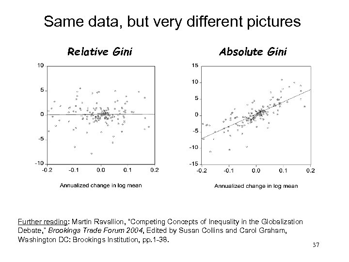
Same data, but very different pictures Relative Gini Absolute Gini Further reading: Martin Ravallion, “Competing Concepts of Inequality in the Globalization Debate, ” Brookings Trade Forum 2004, Edited by Susan Collins and Carol Graham, Washington DC: Brookings Institution, pp. 1 -38. 37
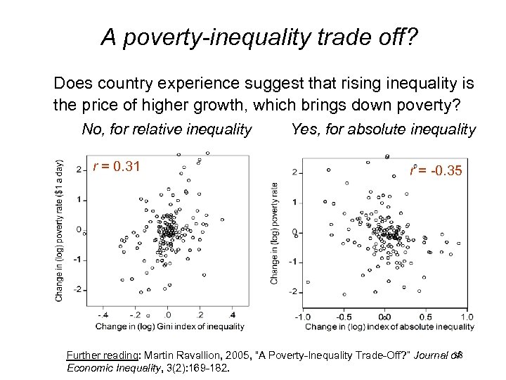
A poverty-inequality trade off? Does country experience suggest that rising inequality is the price of higher growth, which brings down poverty? No, for relative inequality r = 0. 31 Yes, for absolute inequality r = -0. 35 38 Further reading: Martin Ravallion, 2005, “A Poverty-Inequality Trade-Off? ” Journal of Economic Inequality, 3(2): 169 -182.

High inequality is an impediment to pro-poor growth Mean elasticity close to zero in high inequality countries 39

High inequality is an impediment to pro-poor growth • Even when inequality is not changing, it matters to the rate of poverty reduction • It is not the rate of growth that matters, but the distribution-corrected rate of growth Rate of poverty reduction = [constant x (1 - inequality)2 ] x growth rate • Higher levels of inequality have progressively smaller impacts on the elasticity as inequality rises Further reading: Martin Ravallion, “Inequality is Bad for the Poor, ” in Inequality and Poverty Re-Examined, edited by John Micklewright and Steven Jenkins, Oxford: Oxford University 40 Press, forthcoming.

Rate of poverty reduction with a 2% rate of growth in per capita income and a headcount index of 40% • Low-inequality country (Gini=0. 30): the headcount index will be halved in 11 years. • High inequality country (Gini=0. 60): it will then take 35 years to halve the initial poverty rate. • Note: the argument works in reverse: high inequality protects the poor from negative macro shocks. 41

Given these country experiences: What has been happening to inequality in the world as a whole? And what has been happening to poverty? 42

What then has been happening to inequality in the aggregate? “Divergence” vs. “rising (relative) inequality” Fact 1: Poor countries have tended to have lower growth rates over last 40 years or so Fact 2: The between-country component of global inequality has been falling • Both are right: population-weighting is the reason for the difference • Growth in India and (especially) China has been a strong factor in falling between-country inequality. 43

A less unequal world? It´s partly a matter of weights Interpersonal inequality International inequality Inter-country inequality Further reading: Branko Milanovic, Worlds Apart, Princeton University Press 44
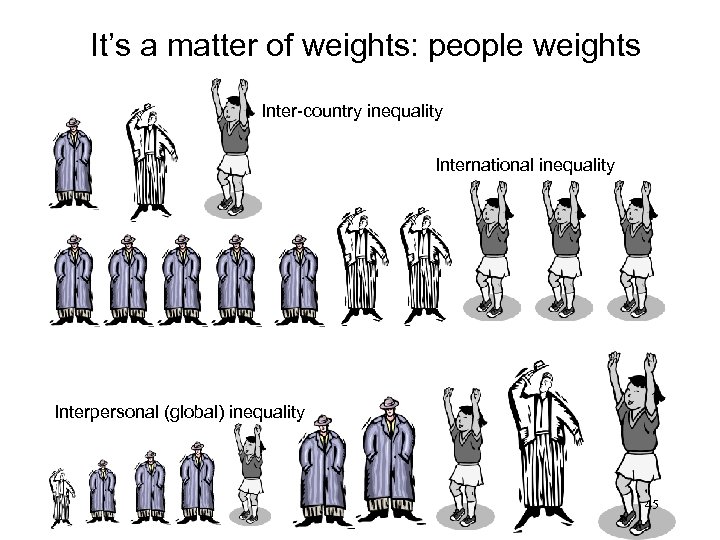
It’s a matter of weights: people weights Inter-country inequality International inequality Interpersonal (global) inequality 45
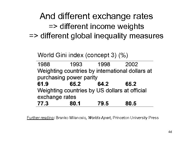
And different exchange rates => different income weights => different global inequality measures World Gini index (concept 3) (%) Further reading: Branko Milanovic, Worlds Apart, Princeton University Press 46
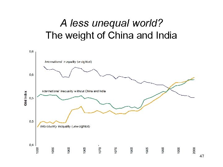
A less unequal world? The weight of China and India 47
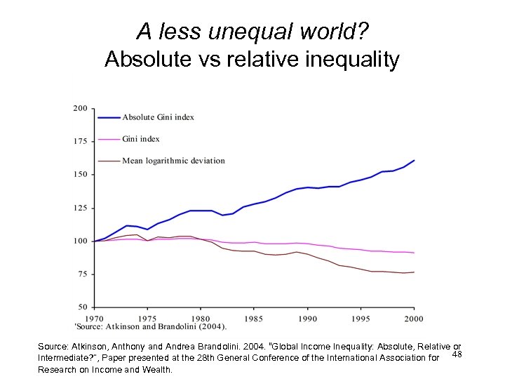
A less unequal world? Absolute vs relative inequality Source: Atkinson, Anthony and Andrea Brandolini. 2004. “Global Income Inequality: Absolute, Relative or Intermediate? ”, Paper presented at the 28 th General Conference of the International Association for 48 Research on Income and Wealth.

Bewteen vs. within country inequality Between-country ineqality has become more important 49

What has been happening to poverty in the aggregate? • With aggregate economic growth in the developing world since 1980 we have seen a trend decline in the incidence of poverty. • Falling absolute numbers of extreme poor (<$1 a day) but rising numbers living between $1 and $2, and little or no progress in reducing the number living under $2 until very recently. 50

Evolution of poverty measures, 1981 -2004 Headcount indices and numbers of poor Source: Shaohua Chen and Martin Ravallion, “Absolute Poverty Measures for the Developing World, ” Policy Research Working Paper 4211, World Bank. 51
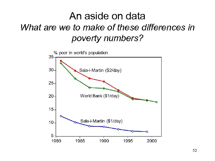
An aside on data What are we to make of these differences in poverty numbers? 52

Aside on data cont. , “We overestimate poverty using surveys, and underestimate its rate of decline” • Two sources of aggregate welfare data: – Private consumption expenditure (PCE) per capita from the national accounts (NAS) – Survey mean consumption or income (from the same surveys used to measure poverty). • Survey mean is typically lower than PCE. • Also signs of divergence over time – Regression coefficient of growth rates = 0. 85 (though not significantly different from one) Further reading: Martin Ravallion, “Measuring Aggregate Welfare in Developing Countries, ” 53 Review of Economics and Statistics, Vol. LXXXV, August 2003, pp. 645 -652.

Aside on data cont. , “We overestimate poverty, . . ” cont. , • So re-calculating the “$/day” poverty measures using NAS for mean (holding relativities constant from the surveys) gives lower (sometimes far lower) poverty counts. • Also tends to gives higher rates of poverty reduction. • Important regional differences – No correlation in EECA – Survey means tend to give higher growth rates in Middle-East and North Africa 54
Aside on data cont. , Surveys are not perfect, but they are the best data for poverty monitoring • Surveys directly measure living standards; national accounts do not. • No reason to think that NAS consumption is more reliable for poverty measurement • Differences in coverage (e. g. , non-profit organizations, financial services) and methods (valuation). • Yes, under-reporting/non-compliance problems, but probably more severe for the rich than the poor. 55

Aside on data cont. , No sound basis for using mean from NAS and distribution from surveys • Poverty = f(mean, distribution) • Why would surveys get the distribution right but the mean wrong, while national accounts get the mean right? • Surveys probably underestimate inequality; NAS overestimate mean consumption of households. • Some survey designs do better than others: – E. g. , consumption surveys are better than income surveys for poverty measurement 56

Aside on data cont. , Survey under-reporting is unlikely to be distribution-neutral: U. S. example Estimates of the percentage adjustments to mean household income needed to allow for non-compliance Further reading: Korinek, Anton, Johan Mistiaen, and Martin Ravallion, 2006. “Survey 57 Nonresponse and the Distribution of Income. ” Journal of Economic Inequality 4(2): 33 -55.
3 Evidence for China and India: The partially awakened giants • Further reading for this section: Shubham Chaudhuri and Martin Ravallion, “Partially Awakened Giants: Uneven Growth in China and India” in Dancing with Giants: China, India, and the Global Economy, edited by L. Alan Winters and Shahid Yusuf, World Bank, 2007. (Also available at: http: //econ. worldbank. org/docsearch. ) 58
Data issues China • Separate urban and rural surveys; comparability problems • Comparability problems over time, esp. , changes in valuation methods in rural household surveys in 1990 (Chen-Ravallion corrections). • Problems with price deflators (esp. , spatial) India • Highly comparable surveys up to 1999/2000 • Changes in survey design in 1999/2000 have created comparability problems. • New survey (2004/05) is comparable to 1993/94 and prior surveys. 59

Growth + poverty reduction in both countries since early 1980 s 60
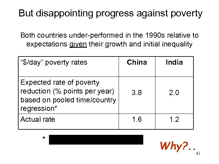
But disappointing progress against poverty Both countries under-performed in the 1990 s relative to expectations given their growth and initial inequality “$/day” poverty rates Expected rate of poverty reduction (% points per year) based on pooled time/country regression* Actual rate * China India 3. 8 2. 0 1. 6 1. 2 Why? . . 61
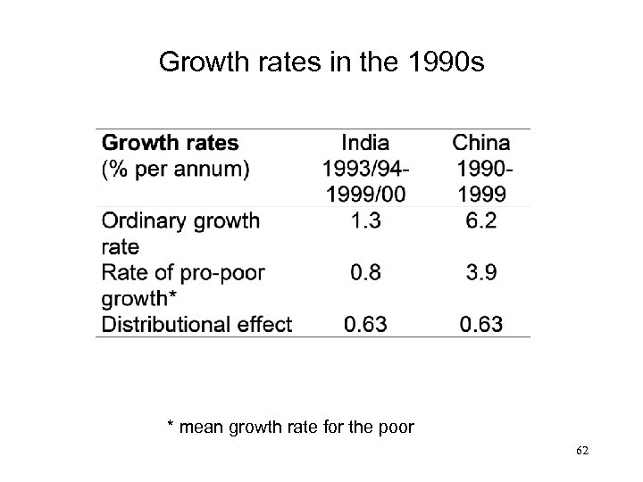
Growth rates in the 1990 s * mean growth rate for the poor 62
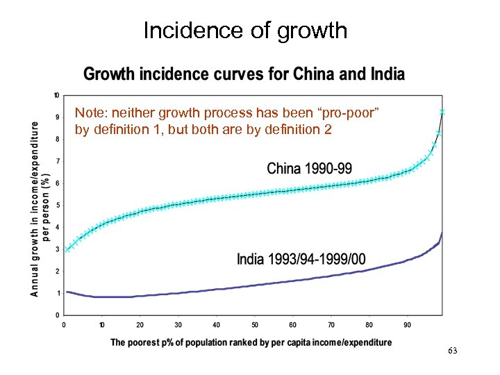
Incidence of growth Note: neither growth process has been “pro-poor” by definition 1, but both are by definition 2 63

Incidence of growth Note: neither growth process has been “pro-poor” by definition 1, but both are by definition 2 64
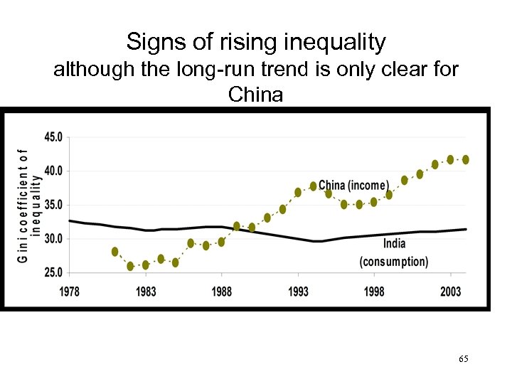
Signs of rising inequality although the long-run trend is only clear for China 65

How uneven is the growth process? What does this mean for poverty and inequality? 66
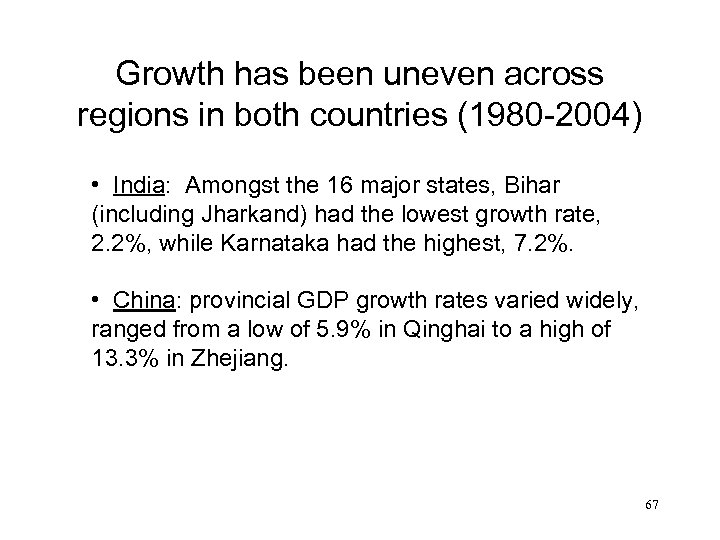
Growth has been uneven across regions in both countries (1980 -2004) • India: Amongst the 16 major states, Bihar (including Jharkand) had the lowest growth rate, 2. 2%, while Karnataka had the highest, 7. 2%. • China: provincial GDP growth rates varied widely, ranged from a low of 5. 9% in Qinghai to a high of 13. 3% in Zhejiang. 67
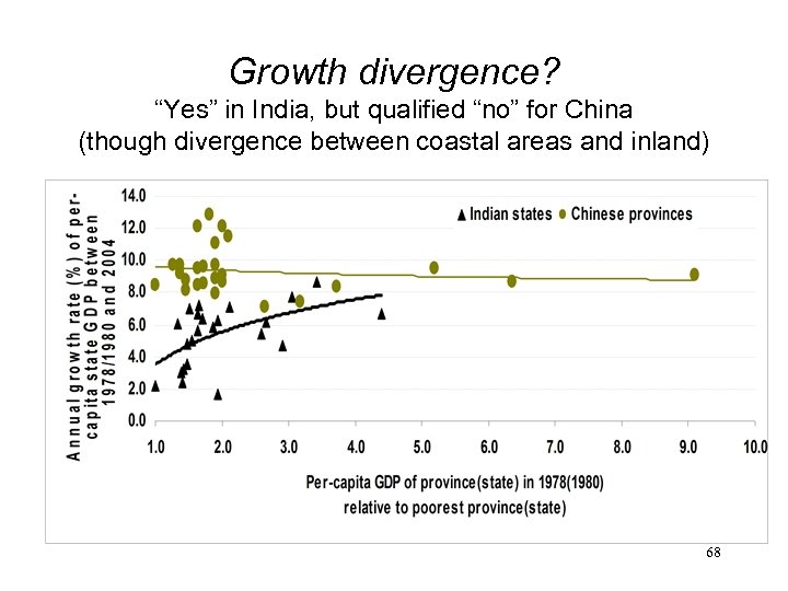
Growth divergence? “Yes” in India, but qualified “no” for China (though divergence between coastal areas and inland) 68
Corresponding unevenness in progress against poverty • China: the coastal areas fared better than inland areas. – The trend rate of decline in the poverty rate between 1981 and 2001 was 8% per year for inland provinces, – versus 17% for the coastal provinces. • India: good performances in poverty reduction in most of the western and southern states—peninsular India (with the exception of AP) • Poor performances in the BIMARU states (Bihar, Madhya Pradesh, Rajasthan and Uttar Pradesh) + the eastern region. 69
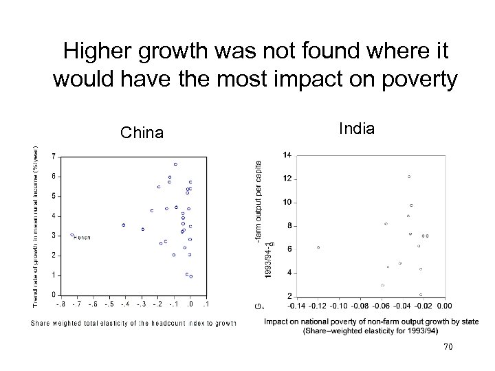
Higher growth was not found where it would have the most impact on poverty China India 70
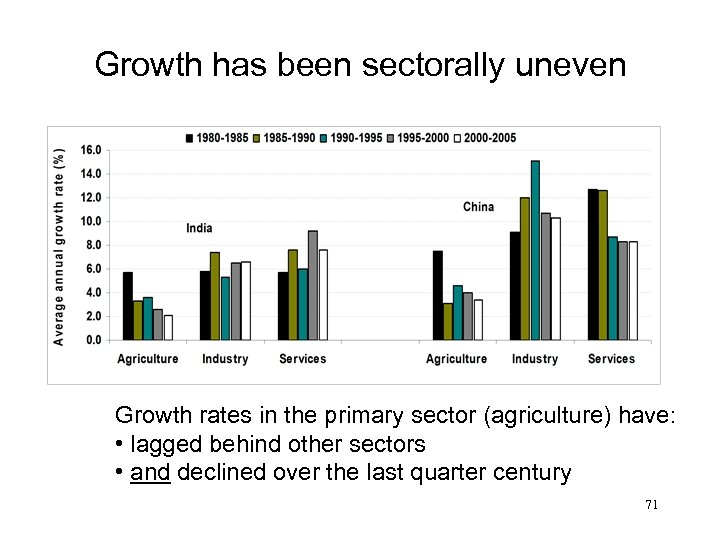
Growth has been sectorally uneven Growth rates in the primary sector (agriculture) have: • lagged behind other sectors • and declined over the last quarter century 71
+ uneven between urban and rural areas • China: trend increase in ratio of urban to rural mean over 1981 -2002 – This is greatly reduced allowing for higher urban inflation rate – But rising trend is still evident since mid-1990 s. • India: trend increase in ratio of urban to rural mean consumption since 1980 s 72
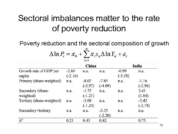
Sectoral imbalances matter to the rate of poverty reduction Poverty reduction and the sectoral composition of growth 73
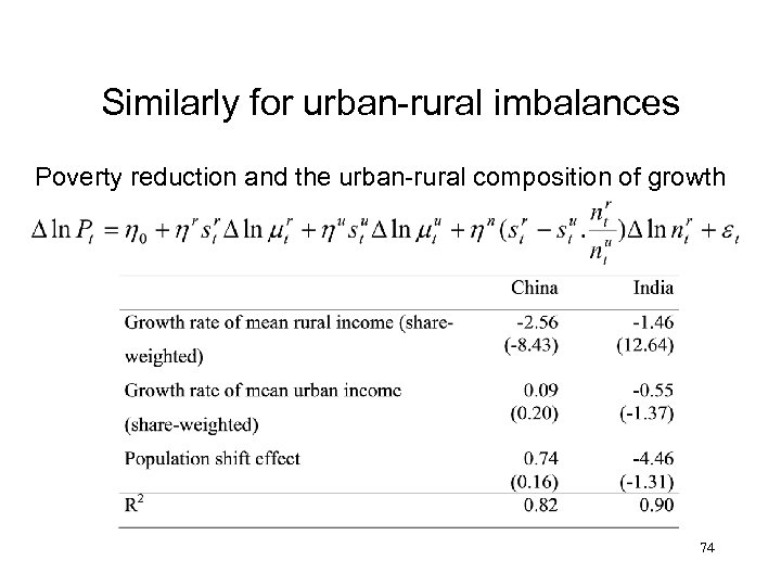
Similarly for urban-rural imbalances Poverty reduction and the urban-rural composition of growth 74

Uneven growth has contributed to rising inequality • Differing initial conditions – Lower land inequality in China – Also lower inequalities in human capital in China – Larger urban-rural inequality in China • China: Primary sector growth has been inequality decreasing; secondary and tertiary have had no effect. • A (moving average) primary-sector growth rate of 7. 0% p. a. would be needed to avoid rising inequality whereas the mean primary-sector growth rate was 75 under 5% between 1981 and 2001.

Why should we care about uneven growth? What should be done about it? 76

Good and bad inequalities • Post-reform development paths of both India and China have been influenced by and have generated both good and bad inequalities. • “Good” or “bad” in terms of what they mean for living standards of the poor 77

Good inequalities • … reflect and reinforce market-based incentives that foster innovation, entrepreneurship and growth • Examples for China – Household Responsibility System: initially inequality reducing, but then inequality increasing forces created – Wage de-compression: higher returns to schooling (from low base) • Examples for India – Greater responsiveness of private investment flows to differences in the investment climate – Exploiting agglomeration economies in industrial location 78
Bad inequalities • … prevent certain segments of the population from escaping poverty. – Geographic poverty traps, patterns of social exclusion, inadequate levels of human capital, lack of access to credit and insurance, corruption and uneven influence • …are rooted in market failures, coordination failures and governance failures • Credit market failures often lie at the root of the problem – it is poor people who tend to be most constrained in financing lumpy investments in human and physical capital. 79

Example 1: Geographic poverty traps • Living in a well-endowed area entails that a poor household can eventually escape poverty, while an otherwise identical household living in a poor area sees stagnation or decline. • In both countries, initially poorer provinces saw lower subsequent growth. • China: Evidence of geographic externalities stemming from both publicly-controlled endowments (such as the density of rural roads) and largely private ones (such as the extent of agricultural development locally). Further reading: Jyotsna Jalan and Martin Ravallion, “Geographic Poverty Traps? A Micro Model of Consumption Growth in Rural China”, Journal of Applied Econometrics Vol. 17(4), pp. 329 -346. 80
Example 2: Inequalities in human capital • …are a key factor impeding pro-poor growth in both countries. • China: Widespread basic schooling at the outset of the reform period • But rising inequalities over time threaten current and future prospects for both growth and poverty reduction. • India: Long-standing inequalities in schooling (higher than in China) that have retarded the pace of poverty reduction at given growth rates, esp. , from non-farm economic growth. * * Gaurav Datt and Martin Ravallion, “Why Has Economic Growth Been More Pro-Poor in Some States 81 of India than Others? ”, Journal of Development Economics Vol. 68 (2002): 381 -400.
Good inequalities can turn into bad ones • Those who benefit initially from the new opportunities can sometimes act to preserve newly realized rents – – • by restricting access to these opportunities or by altering the rules of the game. China: Example of TVEs. Bad inequalities can drive out good ones • Two costs of bad inequalities: – – • Directly reduce growth potential Undermine support for reform Signs that this is happening in both countries 82

Some lessons from sub-national data Performance across India’s states Trend rates of poverty reduction by state (1970 -2000) Further reading for this section: Gaurav Datt and Martin Ravallion, “Has India’s Post-Reform Economic 83 Growth Left the Poor Behind, ”, Journal of Economic Perspectives Vol. 16(3), Summer 2002, pp. 89 -108.
Why has poverty fallen so much faster in some states than others? • Higher average farm yields, higher public spending on development, higher non-farm output and lower inflation were all poverty reducing in India • Agricultural growth, development spending and inflation had similar effects across states • However, the response of poverty to non-farm output growth in India varied significantly between states. 84

India: Elasticities of poverty to non-farm economic growth Kerala WB Elasticities of poverty to non-farm output AP Bihar 85
Higher growth rate in the 1990 s but the rate of poverty reduction is no higher • The poverty impact of higher aggregate growth in the 1990 s has been dulled by its sectoral and geographic composition • The growth has not been found where it would have the greatest impact on poverty 86

Initial conditions matter to the impact of growth on poverty • Low farm productivity, low rural living standards relative to urban areas and poor basic education all inhibited the prospects of the poor participating in growth of India’s non-farm sector. • Rural and human resource development appear to be strongly synergistic with poverty reduction though an expanding non-farm economy. 87

China: Diverse performance across states Trend rates of change in rural headcount index (by province; %/year; 1983 -2001) Fujian, Jiangsu Guangdong Beijing 88

Provinces with higher growth did not have steeper rises in inequality r = -0. 18 89

More unequal provinces faced a double handicap in fighting poverty 1. 2. High inequality provinces had a lower growth elasticity of poverty reduction. High inequality provinces had lower growth: signs of “inefficient inequality” both within rural areas, and between urban and rural areas => 90
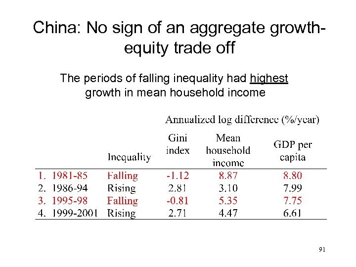
China: No sign of an aggregate growthequity trade off The periods of falling inequality had highest growth in mean household income 91

=> poverty in China would have fallen much faster without rising inequality • If not for the rise in inequality within rural areas, the national poverty rate in 2001 would have been 1. 5% rather than 8%. • Rapidly rising rural inequality meant far lower poverty reduction than one would have expected given the growth. • Nor did higher inequality permit higher growth, over time or across provinces. 92

Steeper increases in inequality did not mean faster poverty reduction 93
4 Conclusions: Some implications for attacking poverty 94

Should policy-makers be worried about rising inequality? • Possibly it is inevitable to some degree. Arthur Lewis: “Development must be inegalitarian because it does not start in every part of the economy at the same time. ” • However, policy makers aiming for pro-poor economic growth should be concerned about the bad inequalities. 95
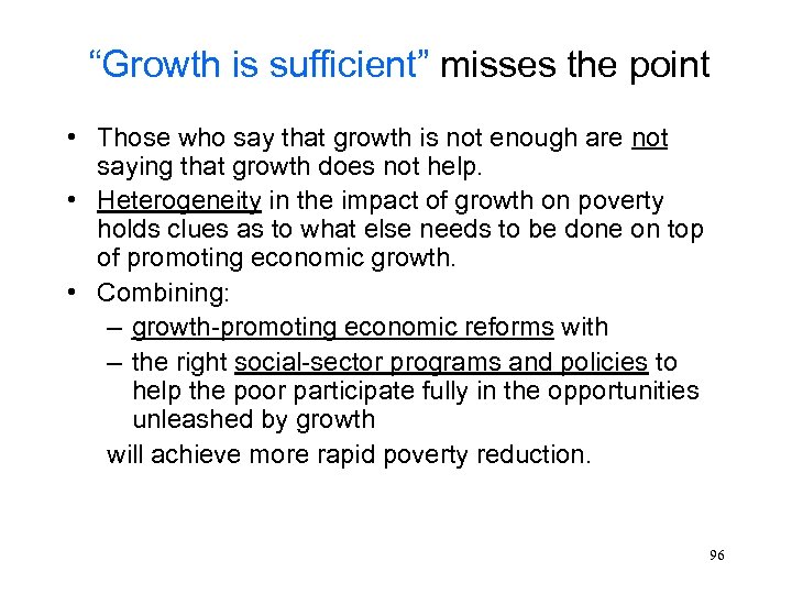
“Growth is sufficient” misses the point • Those who say that growth is not enough are not saying that growth does not help. • Heterogeneity in the impact of growth on poverty holds clues as to what else needs to be done on top of promoting economic growth. • Combining: – growth-promoting economic reforms with – the right social-sector programs and policies to help the poor participate fully in the opportunities unleashed by growth will achieve more rapid poverty reduction. 96
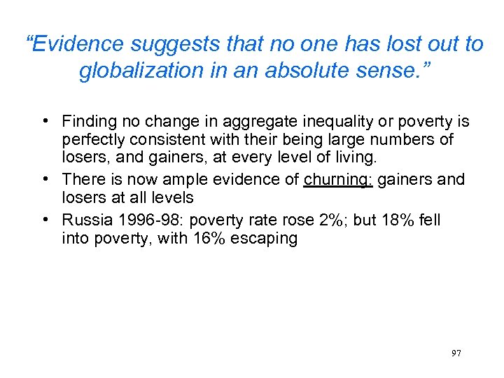
“Evidence suggests that no one has lost out to globalization in an absolute sense. ” • Finding no change in aggregate inequality or poverty is perfectly consistent with their being large numbers of losers, and gainers, at every level of living. • There is now ample evidence of churning: gainers and losers at all levels • Russia 1996 -98: poverty rate rose 2%; but 18% fell into poverty, with 16% escaping 97
Implications for social protection policies • The critics of globalization point to the losers; the supporters point to the gainers. • Policy-makers are unlikely to just maximize aggregate net gains, ignoring distribution • The heterogeneity of impacts holds implications for social protection policies, to help compensate poor losers from policies that are pro-poor overall 98

How to achieve more pro-poor growth? Literature and policy discussions point to the need to: • Develop human and physical assets of poor • Help make markets work better for the poor, esp. , for credit and labor • Removing biases against the poor in public spending, taxation, trade and regulation • Promote agriculture and rural development; invest in local public goods in poor areas • Provide an effective safety net; short term palliative or key instrument for long-term poverty reduction? 99

Monitoring and evaluation • Sensitivity to country context is crucial for assessing what set of policies is pro-poor. • Continuous monitoring of progress and evaluation of specific policies/programs is a crucial input to effective domestic and international efforts against poverty 100
12860080d34296367d268b7d09be0700.ppt