Points and Interval Estimates Example AS Part of

Points and Interval Estimates Example: AS Part of the budgeting process for next year, the manager of the Far Point electric generating plant must estimate the coal he will need for this year. Last year the plant almost ran out, so he is reluctant to budget for the same amount again. The plant manager however does feel that the past usage data will help him estimate that the number of coal to order. A random sample of 10 plant operating weeks chosen over the last 5 years yielded a mean usage of 11, 400 tons a week, a sample sd of 700 tons a week. The plant manager can make a sensible estimate of the amount to order this year including some idea of the accuracy of the estimate he has made.

Points and Interval Estimates 1. Inferences from a Sample 2. Estimation and Confidence Interval 3. Statistical Significance 4. t-statistics 5. Sample Size 6. Finite Population Multiplier

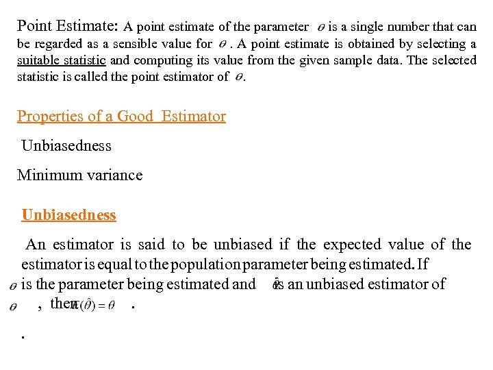Point Estimate: A point estimate of the parameter is a single number that can be regarded as a sensible value for . A point estimate is obtained by selecting a suitable statistic and computing its value from the given sample data. The selected statistic is called the point estimator of . Properties of a Good Estimator Unbiasedness Minimum variance Unbiasedness An estimator is said to be unbiased if the expected value of the estimator is equal to the population parameter being estimated. If is the parameter being estimated and is an unbiased estimator of , then . .

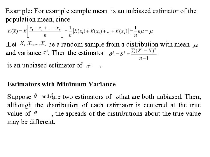Example: For example sample mean is an unbiased estimator of the population mean, since . Let be a random sample from a distribution with mean and variance . Then the estimator is an unbiased estimator of . Estimators with Minimum Variance Suppose are two estimators of that are both unbiased. Then, although the distribution of each estimator is centered at the true value of , the spreads of the distributions about the true value may be different.

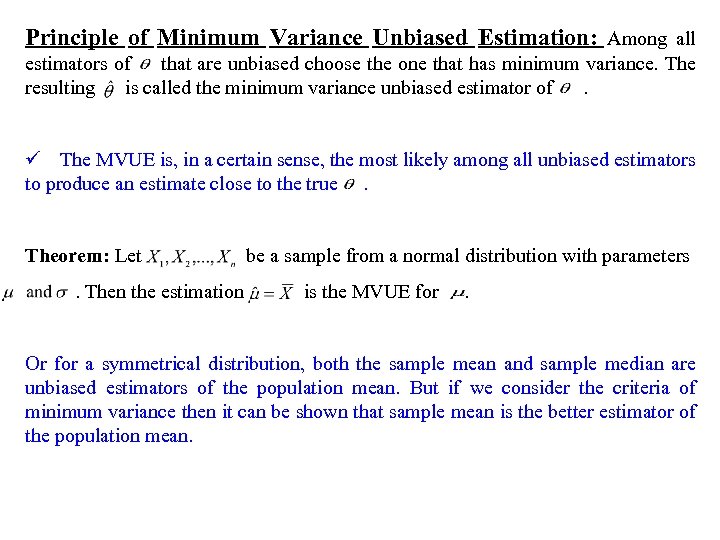Principle of Minimum Variance Unbiased Estimation: Among all estimators of that are unbiased choose the one that has minimum variance. The resulting is called the minimum variance unbiased estimator of . ü The MVUE is, in a certain sense, the most likely among all unbiased estimators to produce an estimate close to the true . Theorem: Let be a sample from a normal distribution with parameters . Then the estimation is the MVUE for . Or for a symmetrical distribution, both the sample mean and sample median are unbiased estimators of the population mean. But if we consider the criteria of minimum variance then it can be shown that sample mean is the better estimator of the population mean.

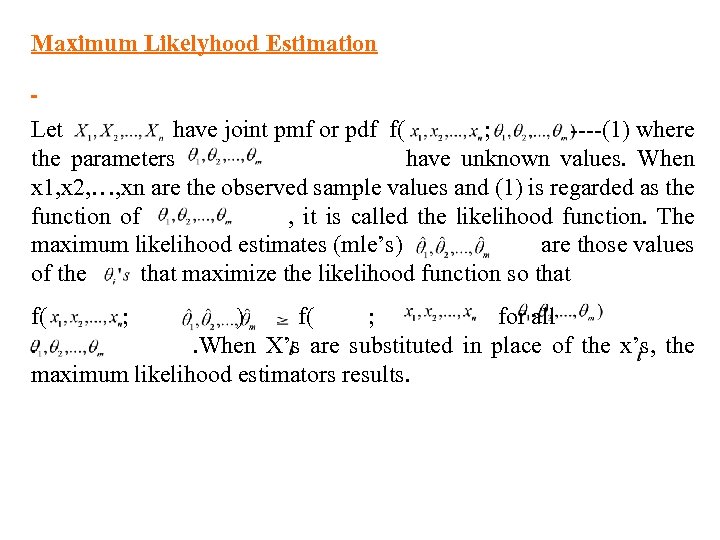Maximum Likelyhood Estimation Let have joint pmf or pdf f( ; ----(1) where the parameters have unknown values. When x 1, x 2, …, xn are the observed sample values and (1) is regarded as the function of , it is called the likelihood function. The maximum likelihood estimates (mle’s) are those values of the that maximize the likelihood function so that f( ; ) f( ; for all . When X’s are substituted in place of the x’s, the maximum likelihood estimators results.

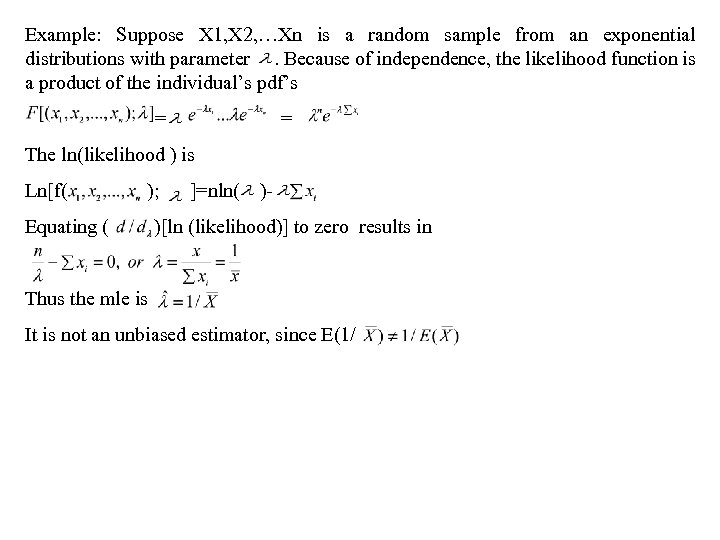Example: Suppose X 1, X 2, …Xn is a random sample from an exponential distributions with parameter . Because of independence, the likelihood function is a product of the individual’s pdf’s = The ln(likelihood ) is Ln[f( ); ]=nln( )- Equating ( )[ln (likelihood)] to zero results in Thus the mle is It is not an unbiased estimator, since E(1/

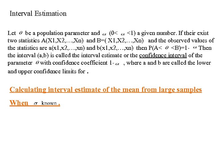Interval Estimation Let be a population parameter and (0< <1) a given number. If their exist two statistics A(X 1, X 2, …, Xn) and B=( X 1, X 2, …, Xn) and the observed values of the statistics are a(x 1, x 2, …, xn) and b(x 1, x 2, …, xn) then P(A<

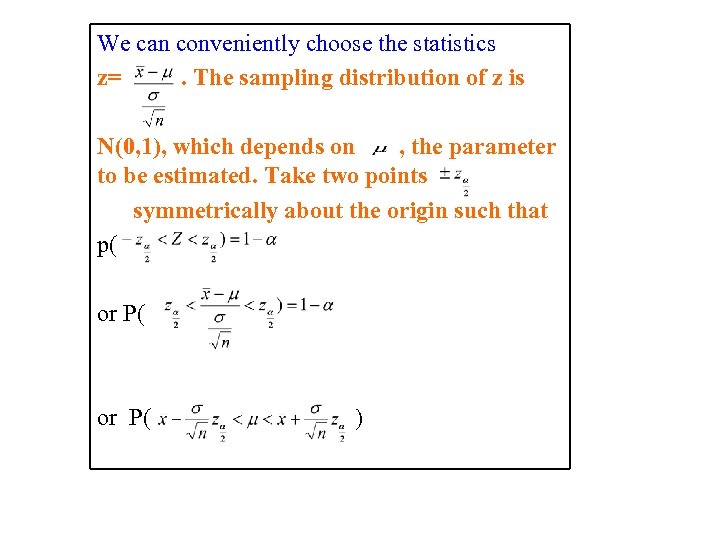We can conveniently choose the statistics z= . The sampling distribution of z is N(0, 1), which depends on , the parameter to be estimated. Take two points symmetrically about the origin such that p( or P( )

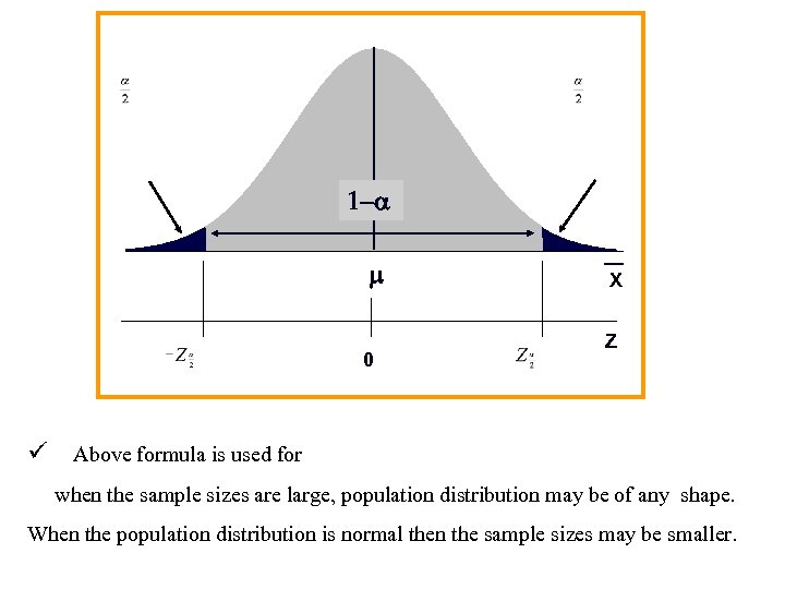1 - m 0 X Z ü Above formula is used for when the sample sizes are large, population distribution may be of any shape. When the population distribution is normal then the sample sizes may be smaller.

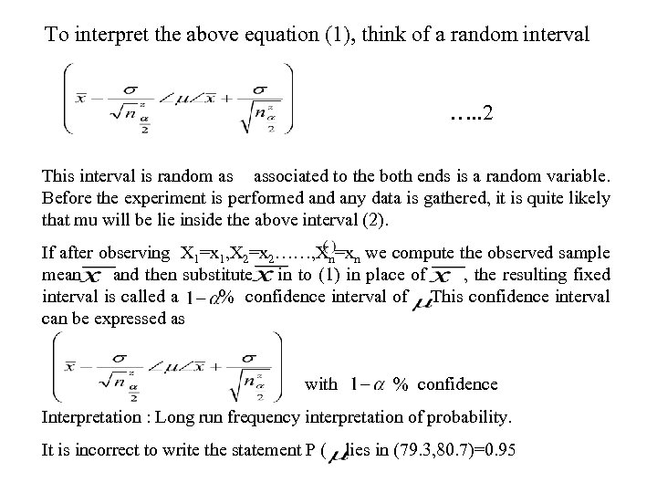To interpret the above equation (1), think of a random interval …. . 2 This interval is random as associated to the both ends is a random variable. Before the experiment is performed any data is gathered, it is quite likely that mu will be lie inside the above interval (2). If after observing X 1=x 1, X 2=x 2……, Xn=xn we compute the observed sample mean and then substitute in to (1) in place of , the resulting fixed interval is called a % confidence interval of This confidence interval can be expressed as with % confidence Interpretation : Long run frequency interpretation of probability. It is incorrect to write the statement P ( lies in (79. 3, 80. 7)=0. 95

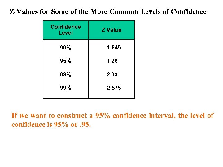Z Values for Some of the More Common Levels of Confidence Level Z Value 90% 1. 645 95% 1. 96 98% 2. 33 99% 2. 575 If we want to construct a 95% confidence interval, the level of confidence is 95% or. 95.

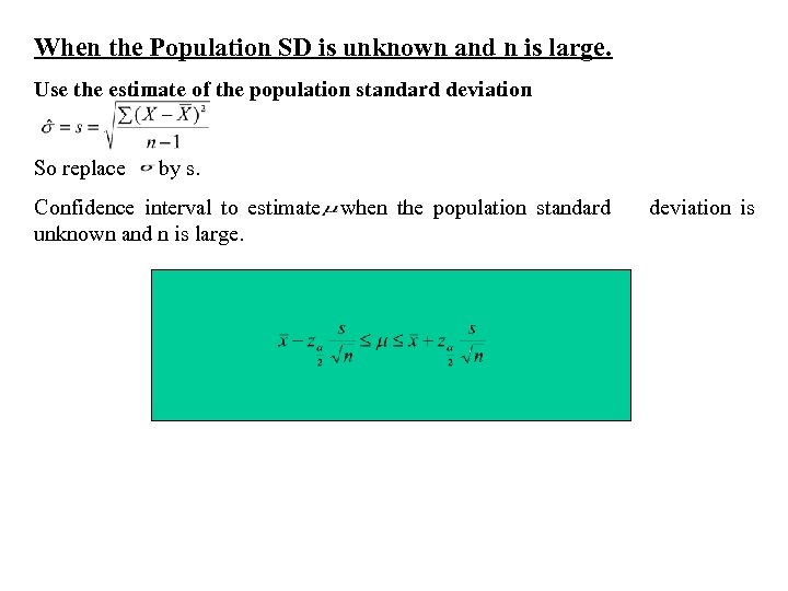When the Population SD is unknown and n is large. Use the estimate of the population standard deviation So replace by s. Confidence interval to estimate when the population standard deviation is unknown and n is large.

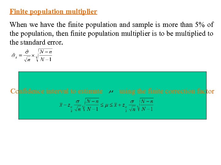Finite population multiplier When we have the finite population and sample is more than 5% of the population, then finite population multiplier is to be multiplied to the standard error. Confidence interval to estimate using the finite correction factor

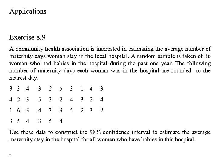Applications Exercise 8. 9 A community health association is interested in estimating the average number of maternity days woman stay in the local hospital. A random sample is taken of 36 woman who had babies in the hospital during the past one year. The following number of maternity days each woman was in the hospital are rounded to the nearest day. 3 3 4 3 2 5 3 1 4 3 4 2 3 5 3 2 4 3 2 4 1 6 3 4 3 3 5 2 3 2 3 5 4 3 5 4 Use these data to construct the 98% confidence interval to estimate the average maternity stay in the hospital for all women who have babies in this hospital.

Estimating the Mean of a Normal Population: Small n and Unknown • The population has a normal distribution. • The value of the population standard deviation is unknown. • The sample size is small, n < 30. • Z distribution is not appropriate for these conditions • t distribution is appropriate

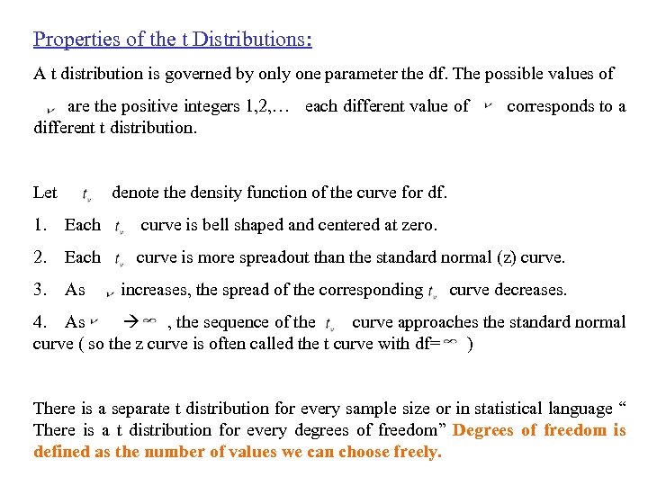Properties of the t Distributions: A t distribution is governed by only one parameter the df. The possible values of are the positive integers 1, 2, … each different value of corresponds to a different t distribution. Let denote the density function of the curve for df. 1. Each curve is bell shaped and centered at zero. 2. Each curve is more spreadout than the standard normal (z) curve. 3. As increases, the spread of the corresponding curve decreases. 4. As , the sequence of the curve approaches the standard normal curve ( so the z curve is often called the t curve with df= ) There is a separate t distribution for every sample size or in statistical language “ There is a t distribution for every degrees of freedom” Degrees of freedom is defined as the number of values we can choose freely.

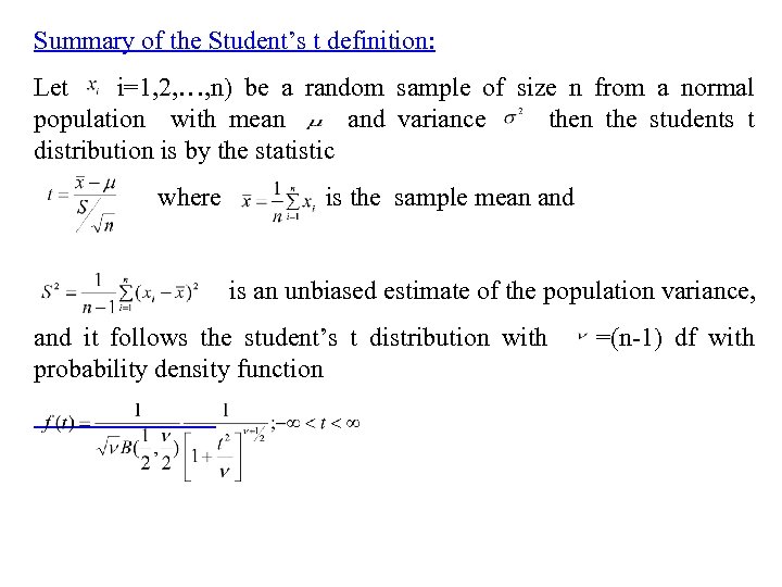Summary of the Student’s t definition: Let i=1, 2, …, n) be a random sample of size n from a normal population with mean and variance then the students t distribution is by the statistic where is the sample mean and is an unbiased estimate of the population variance, and it follows the student’s t distribution with =(n-1) df with probability density function

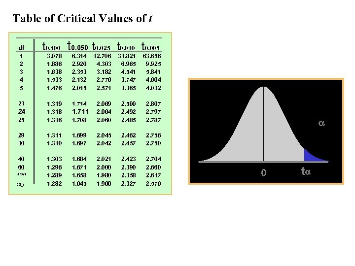Table of Critical Values of t df 1 2 3 4 5 t 0. 100 t 0. 050 t 0. 025 t 0. 010 t 0. 005 3. 078 1. 886 1. 638 1. 533 1. 476 6. 314 2. 920 2. 353 2. 132 2. 015 12. 706 4. 303 3. 182 2. 776 2. 571 31. 821 6. 965 4. 541 3. 747 3. 365 63. 656 9. 925 5. 841 4. 604 4. 032 1. 714 25 1. 319 1. 318 1. 316 1. 708 2. 069 2. 064 2. 060 2. 500 2. 492 2. 485 2. 807 2. 797 2. 787 29 30 1. 311 1. 310 1. 699 1. 697 2. 045 2. 042 2. 462 2. 457 2. 756 2. 750 40 60 120 1. 303 1. 296 1. 289 1. 282 1. 684 1. 671 1. 658 1. 645 2. 021 2. 000 1. 980 1. 960 2. 423 2. 390 2. 358 2. 327 2. 704 2. 660 2. 617 2. 576 23 24 1. 711 t

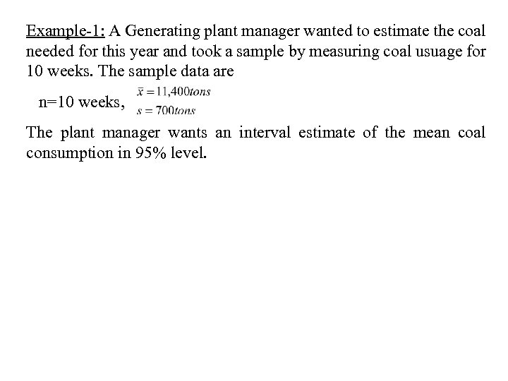Example-1: A Generating plant manager wanted to estimate the coal needed for this year and took a sample by measuring coal usuage for 10 weeks. The sample data are n=10 weeks, The plant manager wants an interval estimate of the mean coal consumption in 95% level.

Exercise 8. 21 The marketing director of a large department store wants to estimate the average number of customers who enters the store every 5 minutes. She randomly selects 5 - minute intervals and count the number of arrivals in the store. She obtains the figure 58, 32, 41, 47, 56, 80, 45, 29, 32 and 78. The analyst assumes the number of arrivals is normally distributed. Using these data, the analyst computes a 95% confidence interval to estimate the mean value for all 5 minutes intervals. What interval values does she get?

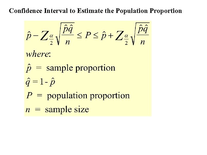Confidence Interval to Estimate the Population Proportion

Exercise 8. 29. The highway department wants to estimate the proportion of vehicle on Interstate 25 between the hours of midnight and 5 am that are 18 wheel tractor trailers. The estimate will be used to determine highway repair and construction consideration and in highway petrol planning. Suppose the researcher for the highway department counted vehicles at different locations on the interstate for several nights during this time period. Of the 3, 481 vehicles counted, 927 were 18 wheelers. a. Determine the point estimate for the proportions of vehicles traveling interstate 25 during this time period that are 18 wheelers. b. Construct a 99 percent confidence interval for the proportions of vehicles on interstate 25 during this time period that are 18 wheelers.

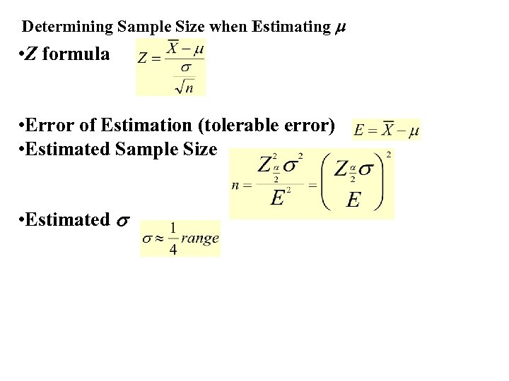Determining Sample Size when Estimating • Z formula • Error of Estimation (tolerable error) • Estimated Sample Size • Estimated

Applications: Exercise: 8. 39 A bank officer wants to determine the amount of average total monthly deposits per customer at the bank. He believes an estimate of this average amount using a confidence interval is sufficient. How large a sample should he take to be within $200 of the actual average with 99% confidence? He assumes the standard deviation of total monthly deposits for all customers is about $1000.

Example 8. 43. What proportion of secretaries of Fortune 500 companies has a personal computer at his or her workstation? You want to answer this question by conducting a random survey. How large a sample should you take if you want to be 95% confident of the results and you want the error of the confidence interval to be no more than. 05? Assume no one has any idea of what the proportion actually is.

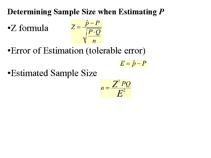Determining Sample Size when Estimating P • Z formula • Error of Estimation (tolerable error) • Estimated Sample Size

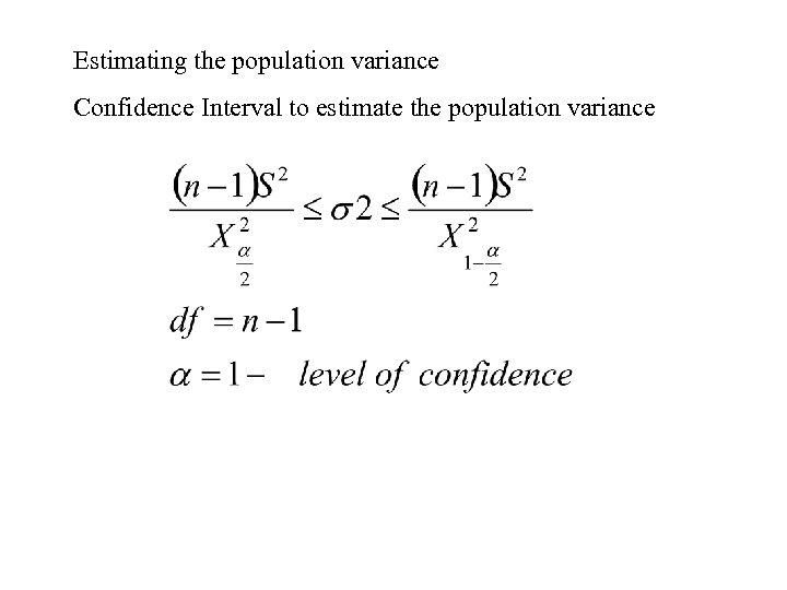Estimating the population variance Confidence Interval to estimate the population variance

Properties of the Chi-square distribution (1) X 2 Distribution is a continuous probability distribution. (2)

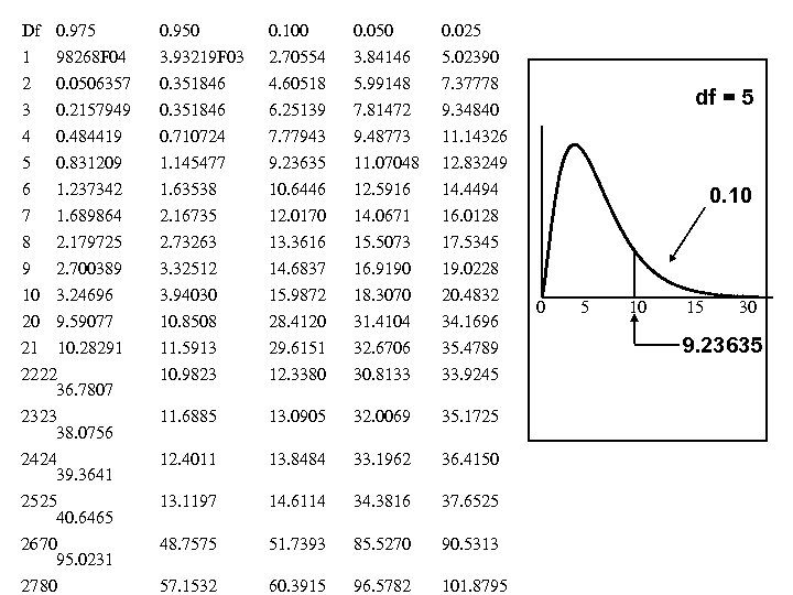Df 0. 975 0. 950 0. 100 0. 050 0. 025 1 2 3 4 98268 F 04 0. 0506357 0. 2157949 0. 484419 3. 93219 F 03 0. 351846 0. 710724 2. 70554 4. 60518 6. 25139 7. 77943 3. 84146 5. 99148 7. 81472 9. 48773 5. 02390 7. 37778 9. 34840 11. 14326 5 6 7 8 9 10 20 0. 831209 1. 237342 1. 689864 2. 179725 2. 700389 3. 24696 9. 59077 1. 145477 1. 63538 2. 16735 2. 73263 3. 32512 3. 94030 10. 8508 9. 23635 10. 6446 12. 0170 13. 3616 14. 6837 15. 9872 28. 4120 11. 07048 12. 5916 14. 0671 15. 5073 16. 9190 18. 3070 31. 4104 12. 83249 14. 4494 16. 0128 17. 5345 19. 0228 20. 4832 34. 1696 11. 5913 10. 9823 29. 6151 12. 3380 32. 6706 30. 8133 35. 4789 33. 9245 11. 6885 13. 0905 32. 0069 35. 1725 12. 4011 13. 8484 33. 1962 36. 4150 13. 1197 14. 6114 34. 3816 37. 6525 48. 7575 51. 7393 85. 5270 90. 5313 57. 1532 60. 3915 96. 5782 101. 8795 21 10. 28291 2222 36. 7807 2323 38. 0756 2424 39. 3641 2525 40. 6465 2670 95. 0231 2780 df = 5 0. 10 0 5 10 15 30 9. 23635

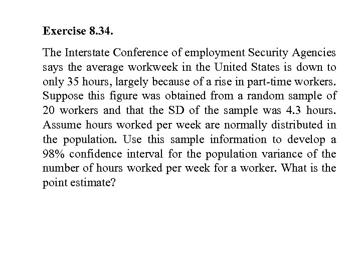Exercise 8. 34. The Interstate Conference of employment Security Agencies says the average workweek in the United States is down to only 35 hours, largely because of a rise in part-time workers. Suppose this figure was obtained from a random sample of 20 workers and that the SD of the sample was 4. 3 hours. Assume hours worked per week are normally distributed in the population. Use this sample information to develop a 98% confidence interval for the population variance of the number of hours worked per week for a worker. What is the point estimate?

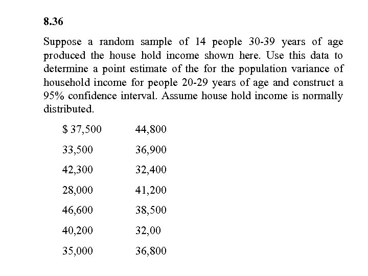8. 36 Suppose a random sample of 14 people 30 -39 years of age produced the house hold income shown here. Use this data to determine a point estimate of the for the population variance of household income for people 20 -29 years of age and construct a 95% confidence interval. Assume house hold income is normally distributed. $ 37, 500 44, 800 33, 500 36, 900 42, 300 32, 400 28, 000 41, 200 46, 600 38, 500 40, 200 32, 00 35, 000 36, 800