Plantwide process control Introduction Sigurd Skogestad NTNU 1

Plantwide process control Introduction Sigurd Skogestad, NTNU 1

Part 1. Plantwide control 2

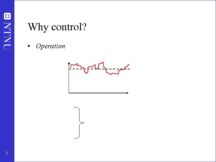Why control? • Operation 3

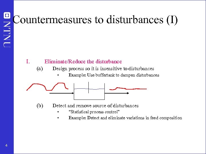Countermeasures to disturbances (I) I. Eliminate/Reduce the disturbance (a) Design process so it is insensitive to disturbances • (b) Detect and remove source of disturbances • • 4 Example: Use buffertank to dampen disturbances “Statistical process control” Example: Detect and eliminate variations in feed composition

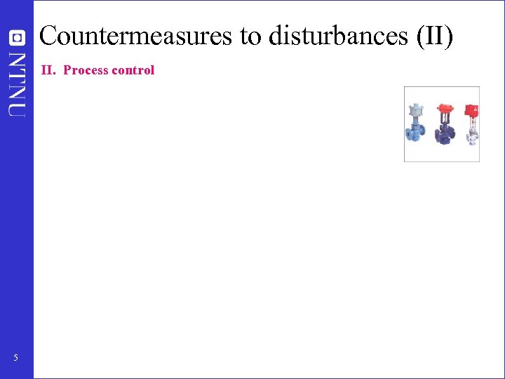Countermeasures to disturbances (II) II. Process control 5

Classification of variables 6

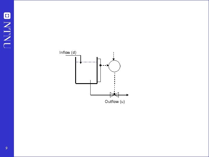
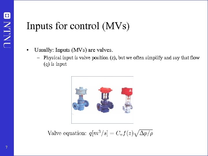Inputs for control (MVs) • Usually: Inputs (MVs) are valves. – Physical input is valve position (z), but we often simplify and say that flow (q) is input 7

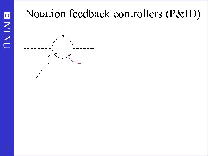Notation feedback controllers (P&ID) 8

Inflow (d) Outflow (u) 9

How we design a control system for a complete chemical plant? • • 10 Where do we start? What should we control? and why? etc.

Plantwide control = Control structure design • Not the tuning and behavior of each control loop, • But rather the control philosophy of the overall plant with emphasis on the structural decisions: – – Selection of controlled variables (“outputs”) Selection of manipulated variables (“inputs”) Selection of (extra) measurements Selection of control configuration (structure of overall controller that interconnects the controlled, manipulated and measured variables) – Selection of controller type (LQG, H-infinity, PID, decoupler, MPC etc. ). • That is: Control structure design includes all the decisions we need make to get from ``PID control’’ to “Ph. D” control 11

Main objectives control system 1. Economics: Implementation of acceptable (near-optimal) operation 2. Regulation: Stable operation ARE THESE OBJECTIVES CONFLICTING? • Usually NOT – Different time scales • Stabilization fast time scale – Stabilization doesn’t “use up” any degrees of freedom • • 14 Reference value (setpoint) available for layer above But it “uses up” part of the time window (frequency range)

Optimal operation (economics) Example of systems we want to operate optimally • Process plant – minimize J=economic cost • Runner – minimize J=time • «Green» process plant – Minimize J=environmental impact (with given economic cost) • General multiobjective: – Min J (scalar cost, often $) – Subject to satisfying constraints (environment, resources) 15

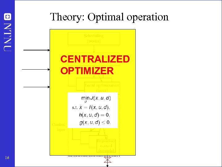Theory: Optimal operation CENTRALIZED OPTIMIZER 16

Practice: Engineering systems • Most (all? ) large-scale engineering systems are controlled using hierarchies of quite simple controllers – Large-scale chemical plant (refinery) – Commercial aircraft • 100’s of loops • Simple components: on-off + PI-control + nonlinear fixes + some feedforward Same in biological systems 17

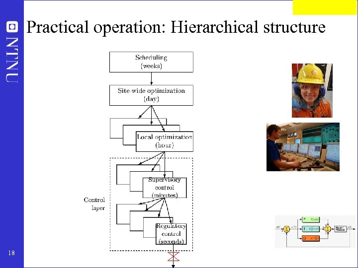Practical operation: Hierarchical structure 18

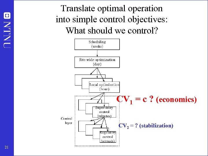Translate optimal operation into simple control objectives: What should we control? CV 1 = c ? (economics) CV 2 = ? (stabilization) 21

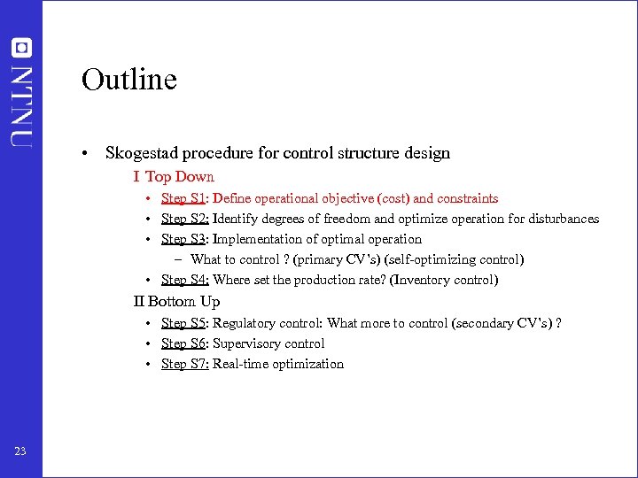Outline • Skogestad procedure for control structure design I Top Down • Step S 1: Define operational objective (cost) and constraints • Step S 2: Identify degrees of freedom and optimize operation for disturbances • Step S 3: Implementation of optimal operation – What to control ? (primary CV’s) (self-optimizing control) • Step S 4: Where set the production rate? (Inventory control) II Bottom Up • Step S 5: Regulatory control: What more to control (secondary CV’s) ? • Step S 6: Supervisory control • Step S 7: Real-time optimization 23

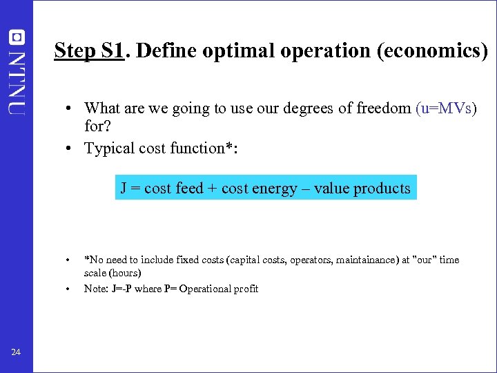Step S 1. Define optimal operation (economics) • What are we going to use our degrees of freedom (u=MVs) for? • Typical cost function*: J = cost feed + cost energy – value products • • 24 *No need to include fixed costs (capital costs, operators, maintainance) at ”our” time scale (hours) Note: J=-P where P= Operational profit

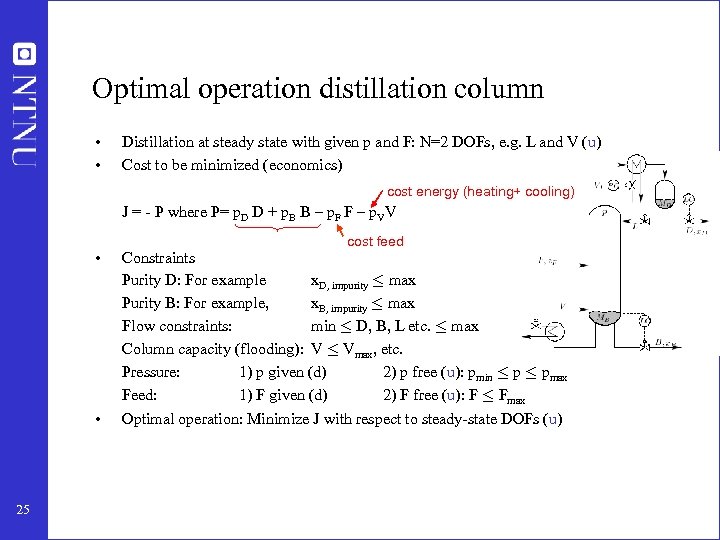Optimal operation distillation column • • Distillation at steady state with given p and F: N=2 DOFs, e. g. L and V (u) Cost to be minimized (economics) cost energy (heating+ cooling) J = - P where P= p. D D + p. B B – p. F F – p. VV • • 25 cost feed Constraints Purity D: For example x. D, impurity · max Purity B: For example, x. B, impurity · max Flow constraints: min · D, B, L etc. · max Column capacity (flooding): V · Vmax, etc. Pressure: 1) p given (d) 2) p free (u): pmin · pmax Feed: 1) F given (d) 2) F free (u): F · Fmax Optimal operation: Minimize J with respect to steady-state DOFs (u)

Step S 2. Optimize (a) Identify degrees of freedom (b) Optimize for expected disturbances • • 26 Need good model, usually steady-state Optimization is time consuming! But it is offline Main goal: Identify ACTIVE CONSTRAINTS A good engineer can often guess the active constraints

Step S 2 a: Degrees of freedom (DOFs) for operation NOT as simple as one may think! To find all operational (dynamic) degrees of freedom: • Count valves! (Nvalves) • “Valves” also includes adjustable compressor power, etc. Anything we can manipulate! BUT: not all these have a (steady-state) effect on the economics 27

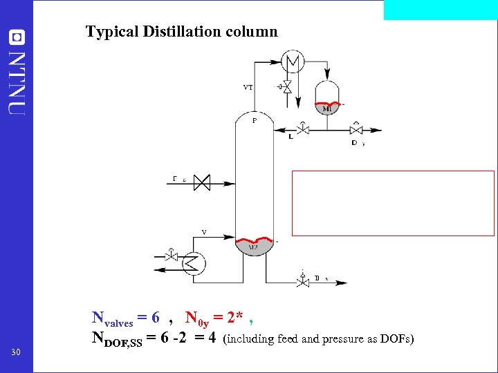Typical Distillation column 30 Nvalves = 6 , N 0 y = 2* , NDOF, SS = 6 -2 = 4 (including feed and pressure as DOFs)

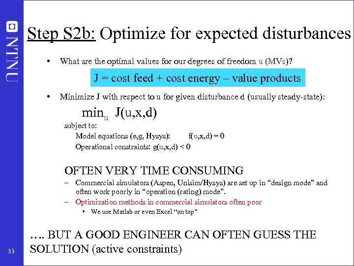Step S 2 b: Optimize for expected disturbances • What are the optimal values for our degrees of freedom u (MVs)? J = cost feed + cost energy – value products • Minimize J with respect to u for given disturbance d (usually steady-state): minu J(u, x, d) subject to: Model equations (e, g, Hysys): f(u, x, d) = 0 Operational constraints: g(u, x, d) < 0 OFTEN VERY TIME CONSUMING – Commercial simulators (Aspen, Unisim/Hysys) are set up in “design mode” and often work poorly in “operation (rating) mode”. – Optimization methods in commercial simulators often poor • We use Matlab or even Excel “on top” 33 …. BUT A GOOD ENGINEER CAN OFTEN GUESS THE SOLUTION (active constraints)

Step S 3: Implementation of optimal operation • Have found the optimal way of operation. How should it be implemented? • What to control ? (primary CV’s). 1. Active constraints 2. Self-optimizing variables (for unconstrained degrees of freedom) 34

Optimal operation - Runner Optimal operation of runner – Cost to be minimized, J=T – One degree of freedom (u=power) – What should we control? 35

Optimal operation - Runner 1. Optimal operation of Sprinter – 100 m. J=T – Active constraint control: • Maximum speed (”no thinking required”) • CV = power (at max) 36

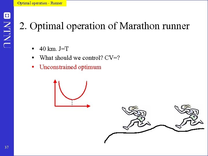Optimal operation - Runner 2. Optimal operation of Marathon runner • 40 km. J=T • What should we control? CV=? • Unconstrained optimum 37

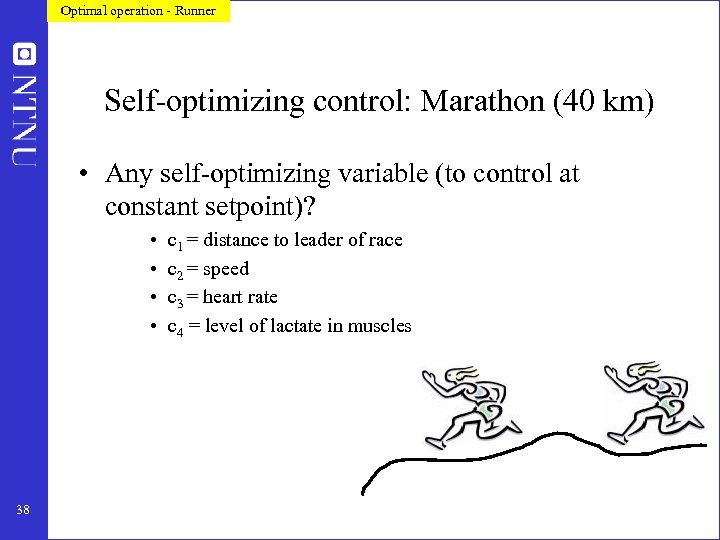Optimal operation - Runner Self-optimizing control: Marathon (40 km) • Any self-optimizing variable (to control at constant setpoint)? • • 38 c 1 = distance to leader of race c 2 = speed c 3 = heart rate c 4 = level of lactate in muscles

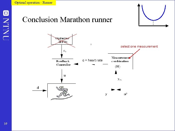Optimal operation - Runner Conclusion Marathon runner select one measurement c = heart rate 39

Step 3. What should we control (c)? (primary controlled variables y 1=c) Selection of controlled variables c 1. Control active constraints! 2. Unconstrained variables: Control self-optimizing variables! 40

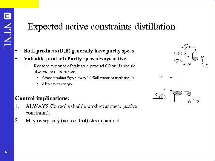Expected active constraints distillation • • Both products (D, B) generally have purity specs Valuable product: Purity spec. always active – Reason: Amount of valuable product (D or B) should always be maximized • Avoid product “give-away” (“Sell water as methanol”) • Also saves energy Control implications: 1. 2. 41 ALWAYS Control valuable product at spec. (active constraint). May overpurify (not control) cheap product

Example with Quiz: Optimal operation of two distillation columns in series 42

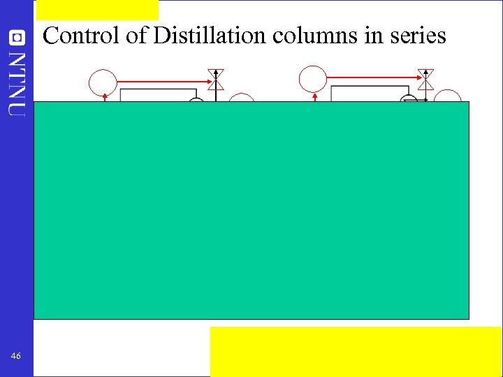
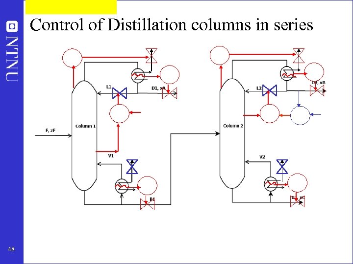
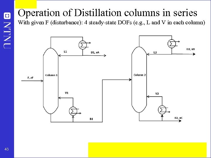Operation of Distillation columns in series With given F (disturbance): 4 steady-state DOFs (e. g. , L and V in each column) 43

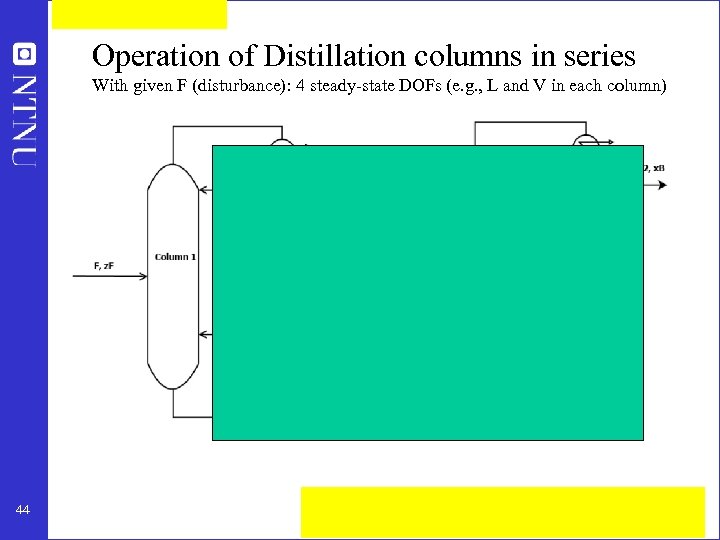Operation of Distillation columns in series With given F (disturbance): 4 steady-state DOFs (e. g. , L and V in each column) 44

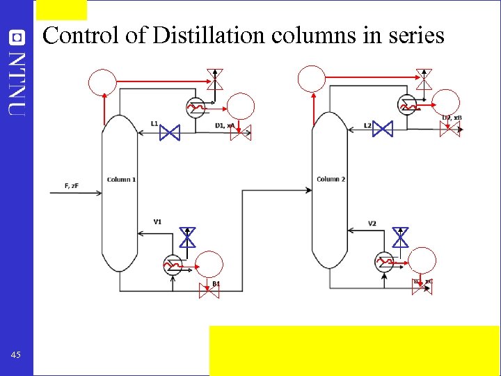Control of Distillation columns in series 45

Control of Distillation columns in series 46

Comment: Distillation column control in practice 47

Control of Distillation columns in series 48

Active constraint regions for two distillation columns in series [$/mol] [mol/s] 49

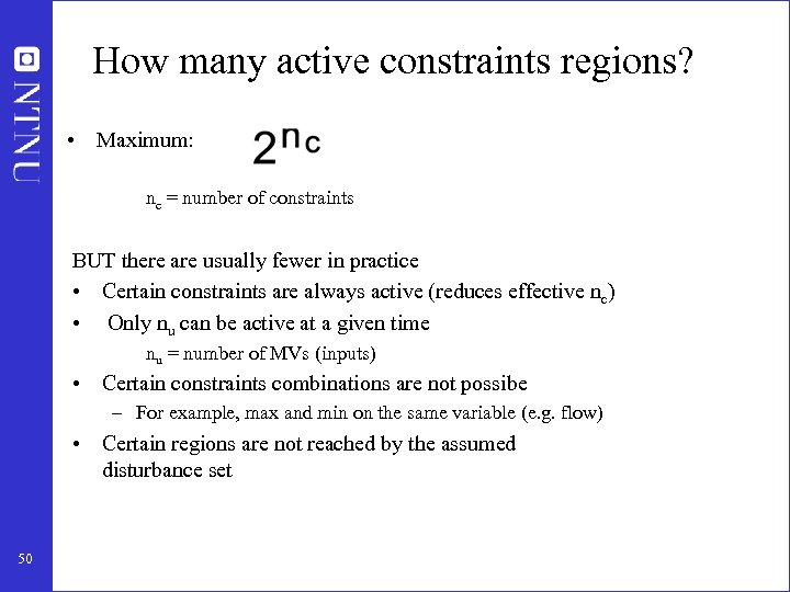How many active constraints regions? • Maximum: nc = number of constraints BUT there are usually fewer in practice • Certain constraints are always active (reduces effective nc) • Only nu can be active at a given time nu = number of MVs (inputs) • Certain constraints combinations are not possibe – For example, max and min on the same variable (e. g. flow) • Certain regions are not reached by the assumed disturbance set 50

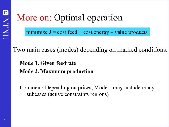More on: Optimal operation minimize J = cost feed + cost energy – value products Two main cases (modes) depending on marked conditions: Mode 1. Given feedrate Mode 2. Maximum production Comment: Depending on prices, Mode 1 may include many subcases (active constraints regions) 51

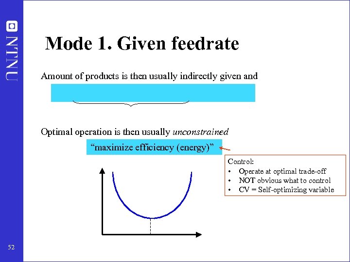Mode 1. Given feedrate Amount of products is then usually indirectly given and Optimal operation is then usually unconstrained “maximize efficiency (energy)” Control: • Operate at optimal trade-off • NOT obvious what to control • CV = Self-optimizing variable 52

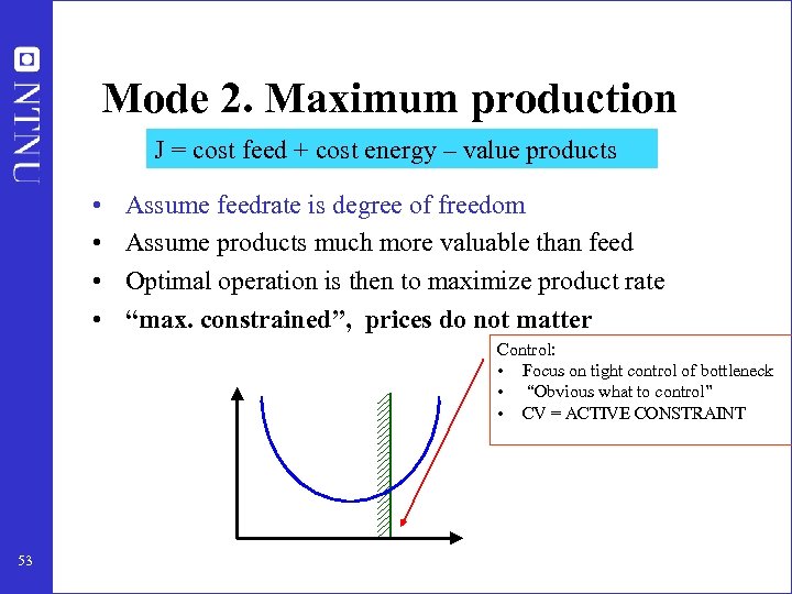Mode 2. Maximum production J = cost feed + cost energy – value products • • Assume feedrate is degree of freedom Assume products much more valuable than feed Optimal operation is then to maximize product rate “max. constrained”, prices do not matter Control: • Focus on tight control of bottleneck • “Obvious what to control” • CV = ACTIVE CONSTRAINT 53

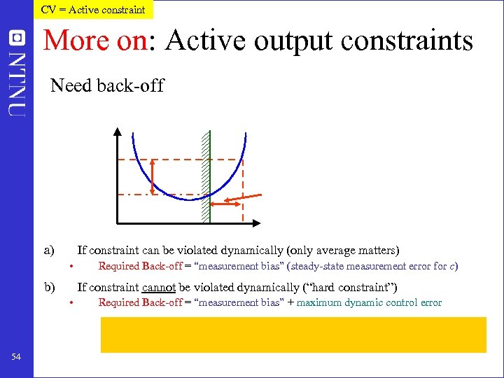CV = Active constraint More on: Active output constraints Need back-off a) If constraint can be violated dynamically (only average matters) • b) If constraint cannot be violated dynamically (“hard constraint”) • 54 Required Back-off = “measurement bias” (steady-state measurement error for c) Required Back-off = “measurement bias” + maximum dynamic control error

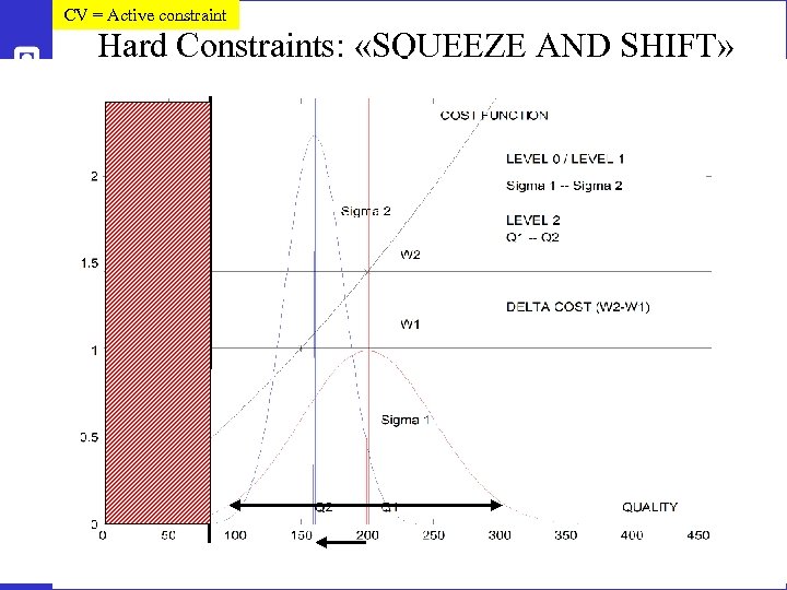CV = Active constraint Hard Constraints: «SQUEEZE AND SHIFT» 55

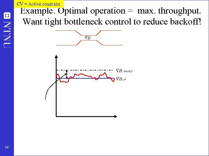CV = Active constraint Example. Optimal operation = max. throughput. Want tight bottleneck control to reduce backoff! 56

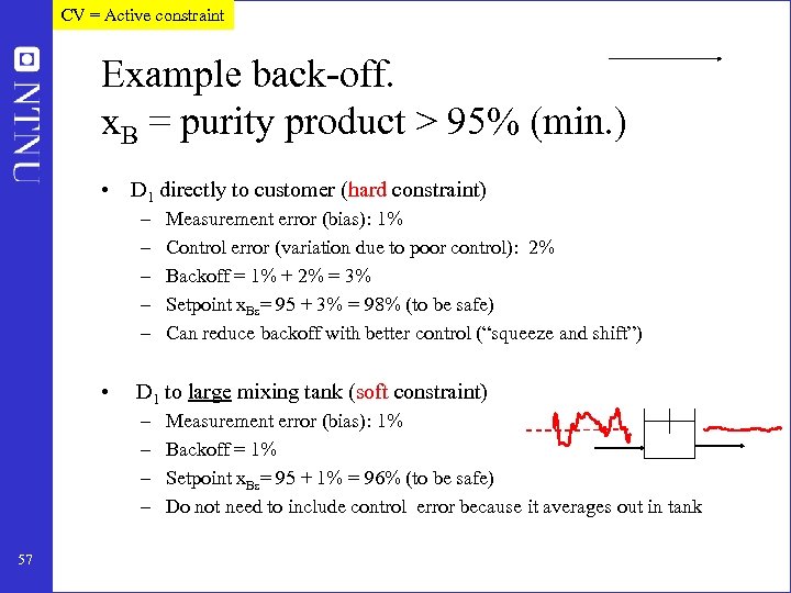CV = Active constraint Example back-off. x. B = purity product > 95% (min. ) • D 1 directly to customer (hard constraint) – – – • D 1 to large mixing tank (soft constraint) – – 57 Measurement error (bias): 1% Control error (variation due to poor control): 2% Backoff = 1% + 2% = 3% Setpoint x. Bs= 95 + 3% = 98% (to be safe) Can reduce backoff with better control (“squeeze and shift”) Measurement error (bias): 1% Backoff = 1% Setpoint x. Bs= 95 + 1% = 96% (to be safe) Do not need to include control error because it averages out in tank

Unconstrained optimum: Control “self-optimizing” variable. • Which variable is best? • Often not obvious (marathon runner) 58

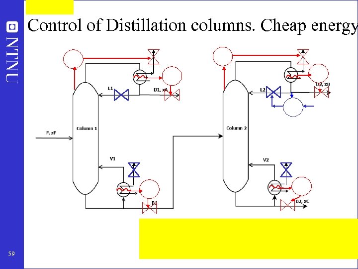Control of Distillation columns. Cheap energy 59

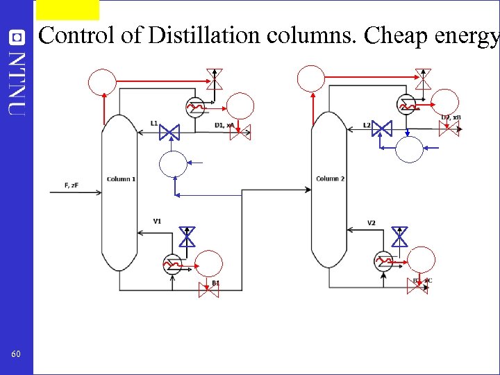Control of Distillation columns. Cheap energy 60

Unconstrained variables More on: WHAT ARE GOOD “SELFOPTIMIZING” VARIABLES? • Intuition: “Dominant variables” (Shinnar) • More precisely 1. Optimal value of CV is constant 2. CV is “sensitive” to MV (large gain) 61

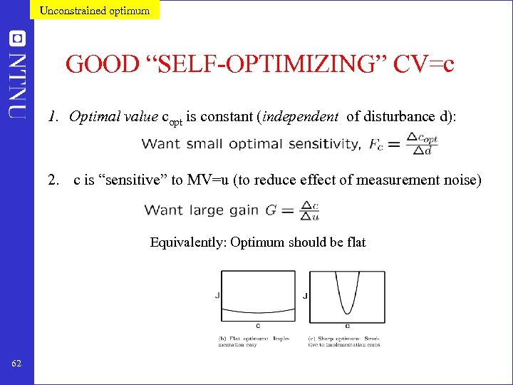Unconstrained optimum GOOD “SELF-OPTIMIZING” CV=c 1. Optimal value copt is constant (independent of disturbance d): 2. c is “sensitive” to MV=u (to reduce effect of measurement noise) Equivalently: Optimum should be flat 62

Conclusion optimal operation ALWAYS: 1. Control active constraints and control them tightly!! – Good times: Maximize throughput -> tight control of bottleneck 2. Identify “self-optimizing” CVs for remaining unconstrained degrees of freedom • Use offline analysis to find expected operating regions and prepare control system for this! – One control policy when prices are low (nominal, unconstrained optimum) – Another when prices are high (constrained optimum = bottleneck) ONLY if necessary: consider RTO on top of this 63