89c5924f8c1a508289677a9e34d06aac.ppt
- Количество слайдов: 64
 Planning Chapter 11. 1 -11. 3 Some material adopted from notes by Andreas Geyer-Schulz and Chuck Dyer
 Overview • What is planning? • Approaches to planning – GPS / STRIPS – Situation calculus formalism [revisited] – Partial-order planning
 Planning problem • Find a sequence of actions that achieves a given goal when executed from a given initial world state • That is, given – a set of operator descriptions defining the possible primitive actions by the agent, – an initial state description, and – a goal state description or predicate, compute a plan, which is – a sequence of operator instances which after executing them in the initial state changes the world to a goal state • Goals are usually specified as a conjunction of goals to be achieved
 Planning vs. problem solving • Planning and problem solving methods can often solve the same sorts of problems • Planning is more powerful and efficient because of the representations and methods used • States, goals, and actions are decomposed into sets of sentences (usually in first-order logic) • Search often proceeds through plan space rather than state space (though there also state-space planners) • Subgoals can be planned independently, reducing the complexity of the planning problem
 Typical assumptions • Atomic time: Each action is indivisible • No concurrent actions allowed, but actions need not be ordered w. r. t each other in the plan • Deterministic actions: action results completely determined — no uncertainty in their effects • Agent is the sole cause of change in the world • Agent is omniscient with complete knowledge of the state of the world • Closed world assumption where everything known to be true in the world is included in the state description and anything not listed is false
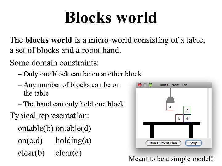 Blocks world The blocks world is a micro-world consisting of a table, a set of blocks and a robot hand. Some domain constraints: – Only one block can be on another block – Any number of blocks can be on the table – The hand can only hold one block Typical representation: ontable(b) ontable(d) on(c, d) holding(a) clear(b) clear(c) Meant to be a simple model!
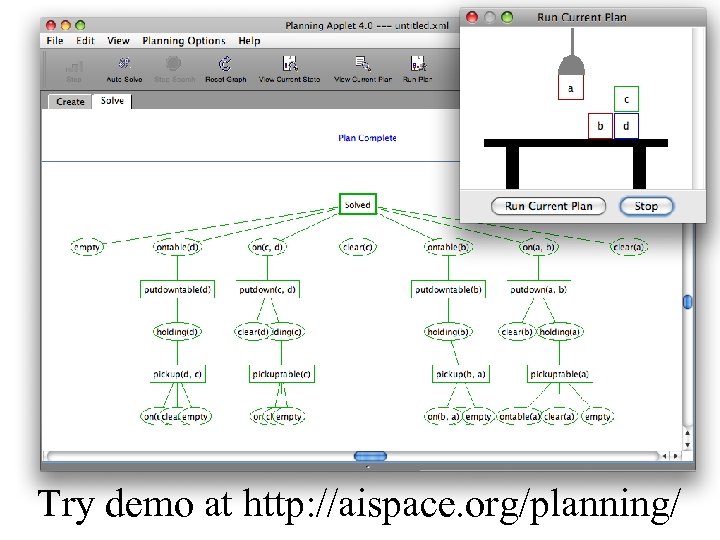 Try demo at http: //aispace. org/planning/
 Major approaches • Planning as search • GPS / STRIPS • Situation calculus • Partial order planning • Hierarchical decomposition (HTN planning) • Planning with constraints (SATplan, Graphplan) • Reactive planning
 Planning as Search • We could think of planning as just another search problem • Actions: generate successor states • States: completely described & only used for successor generation, heuristic fn. evaluation & goal testing. • Goals: represented as a goal test and using a heuristic function • Plan representation: an unbroken sequences of actions forward from initial states (or backward from goal state)
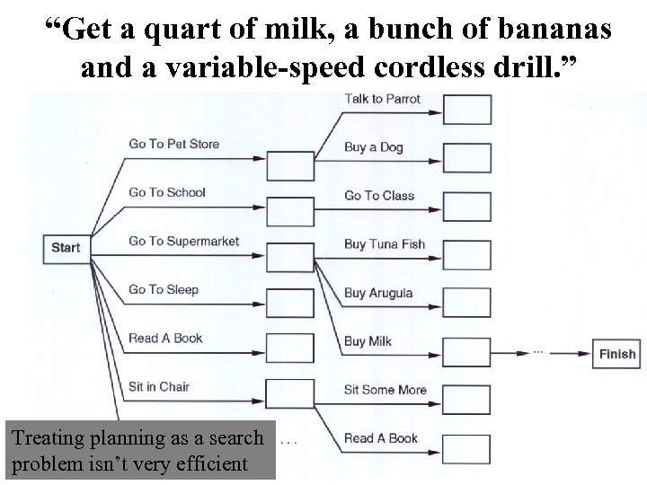 “Get a quart of milk, a bunch of bananas and a variable-speed cordless drill. ” Treating planning as a search problem isn’t very efficient
 General Problem Solver • The General Problem Solver (GPS) system was an early planner (Newell, Shaw, and Simon, 1957) • GPS generated actions that reduced the difference between some state and a goal state • GPS used Means-Ends Analysis – Compare given to desired states; select a best action to do next – A table of differences identifies procedures to reduce types of differences • GPS was a state space planner: it operated in the domain of state space problems specified by an initial state, some goal states, and a set of operations • Introduced a general way to use domain knowledge to select most promising action to take next
 Situation calculus planning • Intuition: Represent the planning problem using first-order logic – Situation calculus lets us reason about changes in the world – Use theorem proving to “prove” that a particular sequence of actions, when applied to the initial situation leads to desired result • This is how the “neats” approach the problem
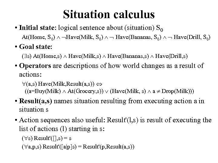 Situation calculus • Initial state: logical sentence about (situation) S 0 At(Home, S 0) Have(Milk, S 0) Have(Bananas, S 0) Have(Drill, S 0) • Goal state: ( s) At(Home, s) Have(Milk, s) Have(Bananas, s) Have(Drill, s) • Operators are descriptions of how world changes as a result of actions: (a, s) Have(Milk, Result(a, s)) ((a=Buy(Milk) At(Grocery, s)) (Have(Milk, s) a Drop(Milk))) • Result(a, s) names situation resulting from executing action a in situation s • Action sequences also useful: Result'(l, s) is result of executing the list of actions (l) starting in s: ( s) Result'([], s) = s ( a, p, s) Result'([a|p]s) = Result'(p, Result(a, s))
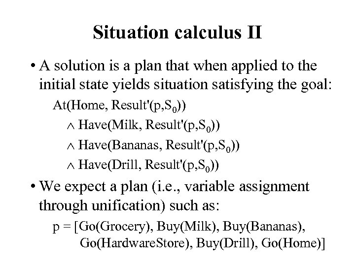 Situation calculus II • A solution is a plan that when applied to the initial state yields situation satisfying the goal: At(Home, Result'(p, S 0)) Have(Milk, Result'(p, S 0)) Have(Bananas, Result'(p, S 0)) Have(Drill, Result'(p, S 0)) • We expect a plan (i. e. , variable assignment through unification) such as: p = [Go(Grocery), Buy(Milk), Buy(Bananas), Go(Hardware. Store), Buy(Drill), Go(Home)]
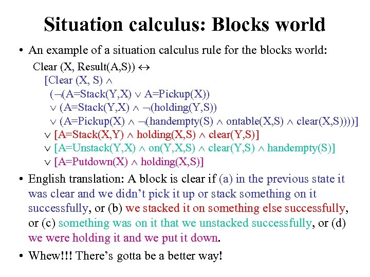 Situation calculus: Blocks world • An example of a situation calculus rule for the blocks world: Clear (X, Result(A, S)) [Clear (X, S) ( (A=Stack(Y, X) A=Pickup(X)) (A=Stack(Y, X) (holding(Y, S)) (A=Pickup(X) (handempty(S) ontable(X, S) clear(X, S))))] [A=Stack(X, Y) holding(X, S) clear(Y, S)] [A=Unstack(Y, X) on(Y, X, S) clear(Y, S) handempty(S)] [A=Putdown(X) holding(X, S)] • English translation: A block is clear if (a) in the previous state it was clear and we didn’t pick it up or stack something on it successfully, or (b) we stacked it on something else successfully, or (c) something was on it that we unstacked successfully, or (d) we were holding it and we put it down. • Whew!!! There’s gotta better way!
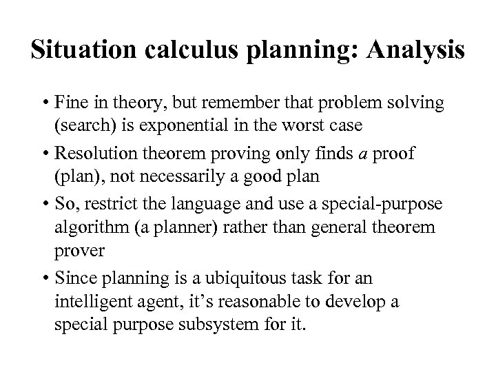 Situation calculus planning: Analysis • Fine in theory, but remember that problem solving (search) is exponential in the worst case • Resolution theorem proving only finds a proof (plan), not necessarily a good plan • So, restrict the language and use a special-purpose algorithm (a planner) rather than general theorem prover • Since planning is a ubiquitous task for an intelligent agent, it’s reasonable to develop a special purpose subsystem for it.
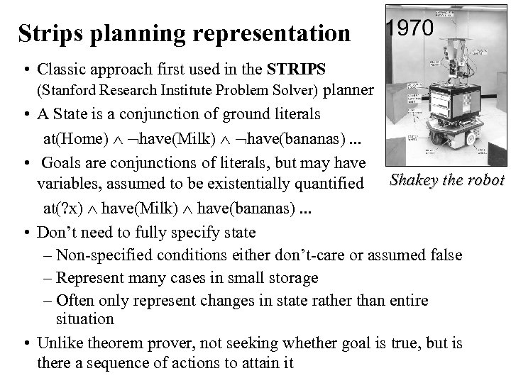 Strips planning representation • Classic approach first used in the STRIPS (Stanford Research Institute Problem Solver) planner • A State is a conjunction of ground literals at(Home) have(Milk) have(bananas). . . • Goals are conjunctions of literals, but may have Shakey the robot variables, assumed to be existentially quantified at(? x) have(Milk) have(bananas). . . • Don’t need to fully specify state – Non-specified conditions either don’t-care or assumed false – Represent many cases in small storage – Often only represent changes in state rather than entire situation • Unlike theorem prover, not seeking whether goal is true, but is there a sequence of actions to attain it
 Shakey video circa 1969 94 M! http: //www. cs. umbc. edu/ai/videos/shakey. avi
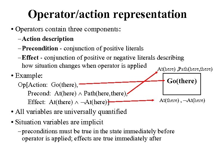 Operator/action representation • Operators contain three components: – Action description – Precondition - conjunction of positive literals – Effect - conjunction of positive or negative literals describing how situation changes when operator is applied At(here) , Path(here, there) • Example: Op[Action: Go(there), Precond: At(here) Path(here, there), Effect: At(there) At(here)] Go(there) At(there) , At(here) • All variables are universally quantified • Situation variables are implicit – preconditions must be true in the state immediately before operator is applied; effects are true immediately after
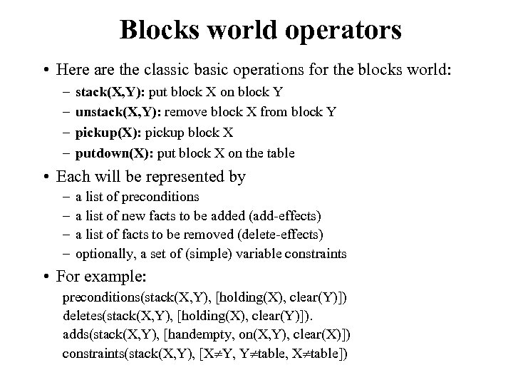 Blocks world operators • Here are the classic basic operations for the blocks world: – – stack(X, Y): put block X on block Y unstack(X, Y): remove block X from block Y pickup(X): pickup block X putdown(X): put block X on the table • Each will be represented by – – a list of preconditions a list of new facts to be added (add-effects) a list of facts to be removed (delete-effects) optionally, a set of (simple) variable constraints • For example: preconditions(stack(X, Y), [holding(X), clear(Y)]) deletes(stack(X, Y), [holding(X), clear(Y)]). adds(stack(X, Y), [handempty, on(X, Y), clear(X)]) constraints(stack(X, Y), [X Y, Y table, X table])
![Blocks world operators (Prolog) operator(unstack(X, Y), operator(stack(X, Y), [on(X, Y), clear(X), handempty], Precond [holding(X), Blocks world operators (Prolog) operator(unstack(X, Y), operator(stack(X, Y), [on(X, Y), clear(X), handempty], Precond [holding(X),](https://present5.com/presentation/89c5924f8c1a508289677a9e34d06aac/image-21.jpg) Blocks world operators (Prolog) operator(unstack(X, Y), operator(stack(X, Y), [on(X, Y), clear(X), handempty], Precond [holding(X), clear(Y)], Add [handempty, on(X, Y), clear(X)], [handempty, clear(X), on(X, Y)], Delete [holding(X), clear(Y)], [X Y, Y table, X table]). Constr [X Y, Y table, X table]). operator(pickup(X), [ontable(X), clear(X), handempty], [holding(X)], [ontable(X), clear(X), handempty], [X table]). operator(putdown(X), [holding(X)], [ontable(X), handempty, clear(X)], [holding(X)], [X table]).
Blocks world operators (Prolog) operator(unstack(X, Y), operator(stack(X, Y), [on(X, Y), clear(X), handempty], Precond [holding(X), clear(Y)], Add [handempty, on(X, Y), clear(X)], [handempty, clear(X), on(X, Y)], Delete [holding(X), clear(Y)], [X Y, Y table, X table]). Constr [X Y, Y table, X table]). operator(pickup(X), [ontable(X), clear(X), handempty], [holding(X)], [ontable(X), clear(X), handempty], [X table]). operator(putdown(X), [holding(X)], [ontable(X), handempty, clear(X)], [holding(X)], [X table]).
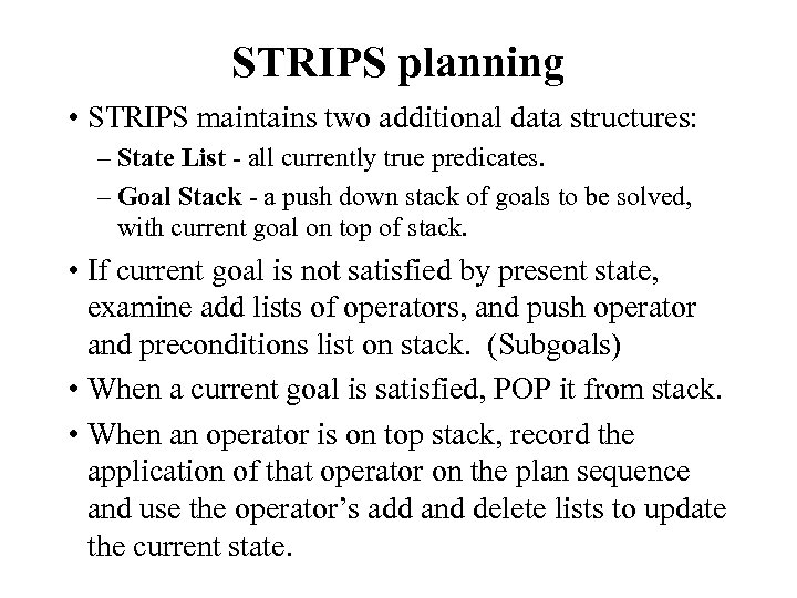 STRIPS planning • STRIPS maintains two additional data structures: – State List - all currently true predicates. – Goal Stack - a push down stack of goals to be solved, with current goal on top of stack. • If current goal is not satisfied by present state, examine add lists of operators, and push operator and preconditions list on stack. (Subgoals) • When a current goal is satisfied, POP it from stack. • When an operator is on top stack, record the application of that operator on the plan sequence and use the operator’s add and delete lists to update the current state.
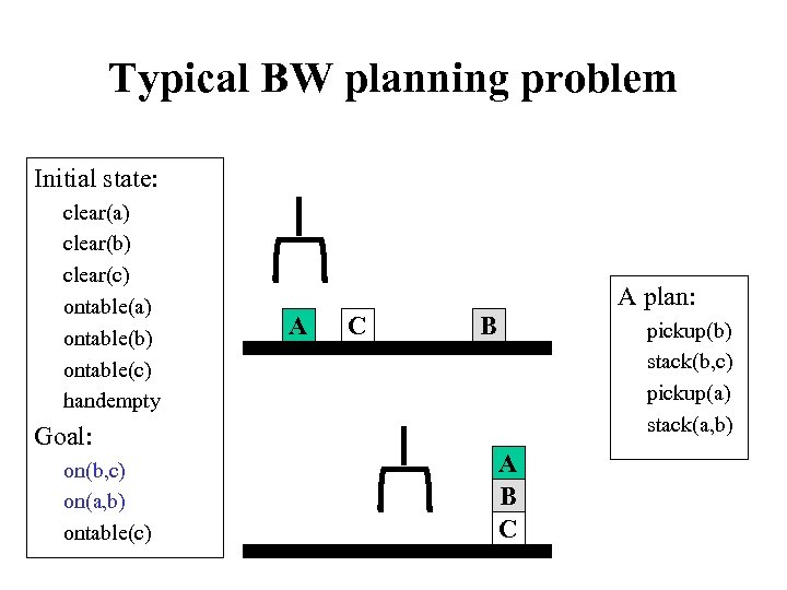 Typical BW planning problem Initial state: clear(a) clear(b) clear(c) ontable(a) ontable(b) ontable(c) handempty Goal: on(b, c) on(a, b) ontable(c) A plan: A C B pickup(b) stack(b, c) pickup(a) stack(a, b) A B C
![Trace (Prolog) strips([on(b, c), on(a, b), ontable(c)], [clear(a), clear(b), clear(c), ontable(a), ontable(b), ontable(c), handempty], Trace (Prolog) strips([on(b, c), on(a, b), ontable(c)], [clear(a), clear(b), clear(c), ontable(a), ontable(b), ontable(c), handempty],](https://present5.com/presentation/89c5924f8c1a508289677a9e34d06aac/image-24.jpg) Trace (Prolog) strips([on(b, c), on(a, b), ontable(c)], [clear(a), clear(b), clear(c), ontable(a), ontable(b), ontable(c), handempty], []) Achieve on(b, c) via stack(b, c) with preconds: [holding(b), clear(c)] strips([holding(b), clear(c)], [clear(a), clear(b), clear(c), ontable(a), ontable(b), ontable(c), handempty], []) Achieve holding(b) via pickup(b) with preconds: [ontable(b), clear(b), handempty] strips([ontable(b), clear(b), handempty], [clear(a), clear(b), clear(c), ontable(a), ontable(b), ontable(c), handempty], []) Applying pickup(b) strips([holding(b), clear(c)], [clear(a), clear(c), holding(b), ontable(a), ontable(c)], [pickup(b)]) Applying stack(b, c) strips([on(b, c), on(a, b), ontable(c)], [handempty, clear(a), clear(b), ontable(a), ontable(c), on(b, c)], [stack(b, c), pickup(b)]) Achieve on(a, b) via stack(a, b) with preconds: [holding(a), clear(b)] strips([holding(a), clear(b)], [handempty, clear(a), clear(b), ontable(a), ontable(c), on(b, c)], [stack(b, c), pickup(b)]) Achieve holding(a) via pickup(a) with preconds: [ontable(a), clear(a), handempty] strips([ontable(a), clear(a), handempty], [handempty, clear(a), clear(b), ontable(a), ontable(c), on(b, c)], [stack(b, c), pickup( b)]) Applying pickup(a) strips([holding(a), clear(b)], [clear(b), holding(a), ontable(c), on(b, c)], [pickup(a), stack(b, c), pickup(b)]) Applying stack(a, b) strips([on(b, c), on(a, b), ontable(c)], [handempty, clear(a), ontable(c), on(a, b), on(b, c)], [stack(a, b), pickup(a), stack(b, c), pickup( b)])
Trace (Prolog) strips([on(b, c), on(a, b), ontable(c)], [clear(a), clear(b), clear(c), ontable(a), ontable(b), ontable(c), handempty], []) Achieve on(b, c) via stack(b, c) with preconds: [holding(b), clear(c)] strips([holding(b), clear(c)], [clear(a), clear(b), clear(c), ontable(a), ontable(b), ontable(c), handempty], []) Achieve holding(b) via pickup(b) with preconds: [ontable(b), clear(b), handempty] strips([ontable(b), clear(b), handempty], [clear(a), clear(b), clear(c), ontable(a), ontable(b), ontable(c), handempty], []) Applying pickup(b) strips([holding(b), clear(c)], [clear(a), clear(c), holding(b), ontable(a), ontable(c)], [pickup(b)]) Applying stack(b, c) strips([on(b, c), on(a, b), ontable(c)], [handempty, clear(a), clear(b), ontable(a), ontable(c), on(b, c)], [stack(b, c), pickup(b)]) Achieve on(a, b) via stack(a, b) with preconds: [holding(a), clear(b)] strips([holding(a), clear(b)], [handempty, clear(a), clear(b), ontable(a), ontable(c), on(b, c)], [stack(b, c), pickup(b)]) Achieve holding(a) via pickup(a) with preconds: [ontable(a), clear(a), handempty] strips([ontable(a), clear(a), handempty], [handempty, clear(a), clear(b), ontable(a), ontable(c), on(b, c)], [stack(b, c), pickup( b)]) Applying pickup(a) strips([holding(a), clear(b)], [clear(b), holding(a), ontable(c), on(b, c)], [pickup(a), stack(b, c), pickup(b)]) Applying stack(a, b) strips([on(b, c), on(a, b), ontable(c)], [handempty, clear(a), ontable(c), on(a, b), on(b, c)], [stack(a, b), pickup(a), stack(b, c), pickup( b)])
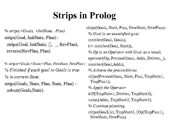 Strips in Prolog strips(Goals, State, Plan, New. State, New. Plan): % strips(+Goals, +Init. State, -Plan) % Goal is an unsatisfied goal. strips(Goal, Init. State, Plan): member(Goal, Goals), strips(Goal, Init. State, [], _, Rev. Plan), (+ member(Goal, State)), reverse(Rev. Plan, Plan). % Op is an Operator with Goal as a result. operator(Op, Preconditions, Adds, Deletes, _), % strips(+Goals, +State, +Plan, -New. State, New. Plan ) member(Goal, Adds), % Finished if each goal in Goals is true % Achieve the preconditions strips(Preconditions, State, Plan, Tmp. State 1, % in current State. Tmp. Plan 1), strips(Goals, State, Plan) : % Apply the Operator subset(Goals, State). diff(Tmp. State 1, Deletes, Tmp. State 2), union(Adds, Tmp. State 2, Tmp. State 3). % Continue planning. strips(Goal. List, Tmp. State 3, [Op|Tmp. Plan 1], New. State, New. Plan).
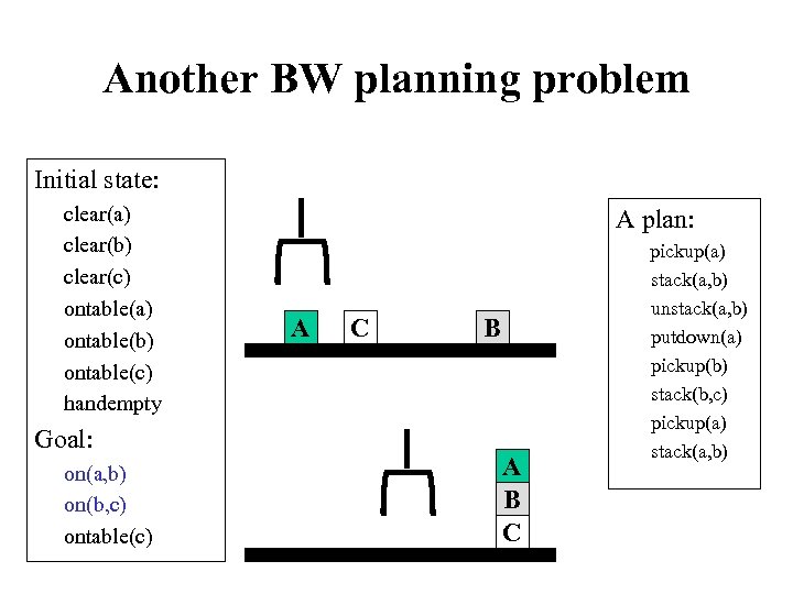 Another BW planning problem Initial state: clear(a) clear(b) clear(c) ontable(a) ontable(b) ontable(c) handempty Goal: on(a, b) on(b, c) ontable(c) A plan: A C B A B C pickup(a) stack(a, b) unstack(a, b) putdown(a) pickup(b) stack(b, c) pickup(a) stack(a, b)
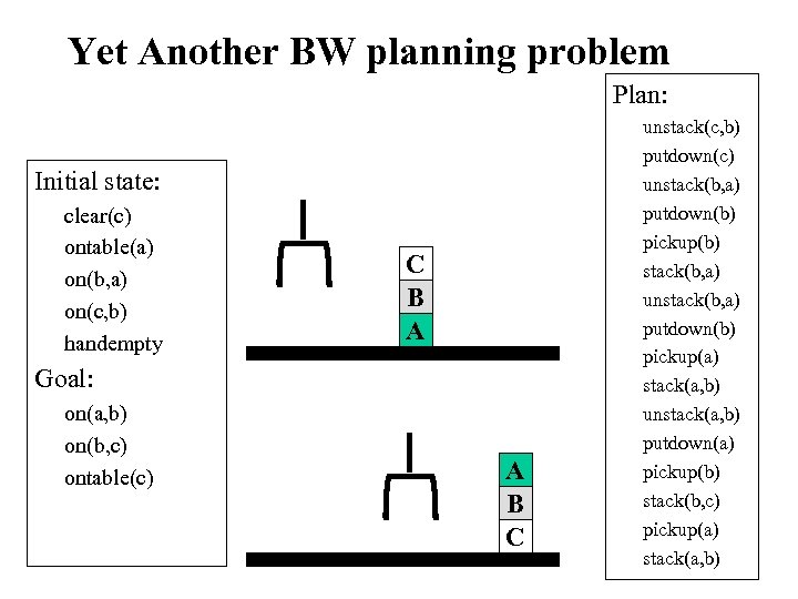 Yet Another BW planning problem Plan: Initial state: clear(c) ontable(a) on(b, a) on(c, b) handempty C B A Goal: on(a, b) on(b, c) ontable(c) A B C unstack(c, b) putdown(c) unstack(b, a) putdown(b) pickup(b) stack(b, a) unstack(b, a) putdown(b) pickup(a) stack(a, b) unstack(a, b) putdown(a) pickup(b) stack(b, c) pickup(a) stack(a, b)
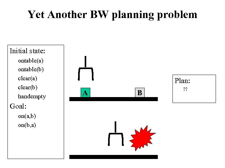 Yet Another BW planning problem Initial state: ontable(a) ontable(b) clear(a) clear(b) handempty Goal: on(a, b) on(b, a) Plan: A B ? ?
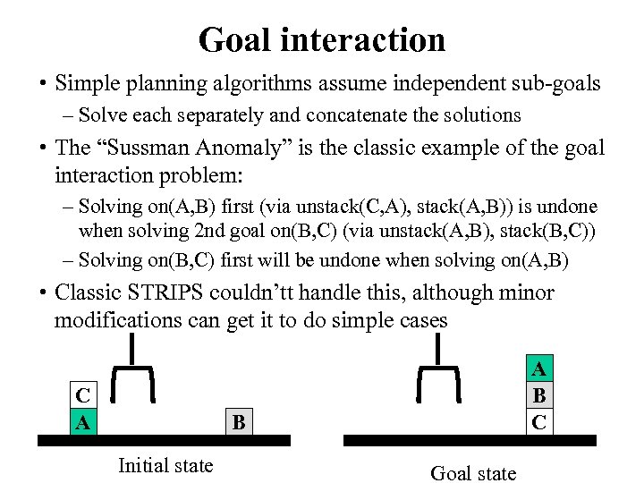 Goal interaction • Simple planning algorithms assume independent sub-goals – Solve each separately and concatenate the solutions • The “Sussman Anomaly” is the classic example of the goal interaction problem: – Solving on(A, B) first (via unstack(C, A), stack(A, B)) is undone when solving 2 nd goal on(B, C) (via unstack(A, B), stack(B, C)) – Solving on(B, C) first will be undone when solving on(A, B) • Classic STRIPS couldn’tt handle this, although minor modifications can get it to do simple cases C A A B C B Initial state Goal state
![Sussman Anomaly Achieve on(a, b) via stack(a, b) with preconds: [holding(a), clear(b)] |Achieve holding(a) Sussman Anomaly Achieve on(a, b) via stack(a, b) with preconds: [holding(a), clear(b)] |Achieve holding(a)](https://present5.com/presentation/89c5924f8c1a508289677a9e34d06aac/image-30.jpg) Sussman Anomaly Achieve on(a, b) via stack(a, b) with preconds: [holding(a), clear(b)] |Achieve holding(a) via pickup(a) with preconds: [ontable(a), clear(a), handempty] ||Achieve clear(a) via unstack(_1584, a) with preconds: [on(_1584, a), clear(_1584), handempty] ||Applying unstack(c, a) ||Achieve handempty via putdown(_2691) with preconds: [holding(_2691)] ||Applying putdown(c) |Applying pickup(a) Applying stack(a, b) Achieve on(b, c) via stack(b, c) with preconds: [holding(b), clear(c)] |Achieve holding(b) via pickup(b) with preconds: [ontable(b), clear(b), handempty] ||Achieve clear(b) via unstack(_5625, b) with preconds: [on(_5625, b), clear(_5625), handempty] ||Applying unstack(a, b) ||Achieve handempty via putdown(_6648) with preconds: [holding(_6648)] ||Applying putdown(a) |Applying pickup(b) Applying stack(b, c) Achieve on(a, b) via stack(a, b) with preconds: [holding(a), clear(b)] |Achieve holding(a) via pickup(a) with preconds: [ontable(a), clear(a), handempty] |Applying pickup(a) Applying stack(a, b) C A Initial state B From [clear(b), clear(c), ontable(a), ontable(b), on( c, a), handempty] To [on(a, b), on(b, c), ontable(c)] Do: unstack(c, a) putdown(c) pickup(a) stack(a, b) unstack(a, b) putdown(a) pickup(b) stack(b, c) pickup(a) stack(a, b) Goal state A B C
Sussman Anomaly Achieve on(a, b) via stack(a, b) with preconds: [holding(a), clear(b)] |Achieve holding(a) via pickup(a) with preconds: [ontable(a), clear(a), handempty] ||Achieve clear(a) via unstack(_1584, a) with preconds: [on(_1584, a), clear(_1584), handempty] ||Applying unstack(c, a) ||Achieve handempty via putdown(_2691) with preconds: [holding(_2691)] ||Applying putdown(c) |Applying pickup(a) Applying stack(a, b) Achieve on(b, c) via stack(b, c) with preconds: [holding(b), clear(c)] |Achieve holding(b) via pickup(b) with preconds: [ontable(b), clear(b), handempty] ||Achieve clear(b) via unstack(_5625, b) with preconds: [on(_5625, b), clear(_5625), handempty] ||Applying unstack(a, b) ||Achieve handempty via putdown(_6648) with preconds: [holding(_6648)] ||Applying putdown(a) |Applying pickup(b) Applying stack(b, c) Achieve on(a, b) via stack(a, b) with preconds: [holding(a), clear(b)] |Achieve holding(a) via pickup(a) with preconds: [ontable(a), clear(a), handempty] |Applying pickup(a) Applying stack(a, b) C A Initial state B From [clear(b), clear(c), ontable(a), ontable(b), on( c, a), handempty] To [on(a, b), on(b, c), ontable(c)] Do: unstack(c, a) putdown(c) pickup(a) stack(a, b) unstack(a, b) putdown(a) pickup(b) stack(b, c) pickup(a) stack(a, b) Goal state A B C
 Sussman Anomaly • Classic Strips assumed that once a goal had been satisfied it would stay satisfied. • Our simple Prolog version selects any currently unsatisfied goal to tackle at each iteration. • This can handle this problem, at the expense of looping for other problems. • What’s needed? -- a notion of “protecting” a subgoal so that it isn’t undone by some later step.
 State-space planning • STRIPS searches thru a space of situations (where you are, what you have, etc. ) – Plan is a solution found by “searching” through the situations to get to the goal • Progression planners search forward from initial state to goal state – Usually results in a high branching factor • Regression planners search backward from goal – OK if operators have enough information to go both ways – Ideally this leads to reduced branching –you are only considering things that are relevant to the goal – Handling a conjunction of goals is difficult (e. g. , STRIPS)
 Some example domains • We’ll use some simple problems with a real world flavor to illustrate planning problems and algorithms • Putting on your socks and hoes in the morning – Actions like put-on-left-sock, put-on-right-shoe • Planning a shopping trip involving buying several kinds of items – Actions like go(X), buy(Y)
 Plan-space planning • An alternative is to search through the space of plans, rather than situations • Start from a partial plan which is expanded and refined until a complete plan is generated • Refinement operators add constraints to the partial plan and modification operators for other changes • We can still use STRIPS-style operators: Op(ACTION: Right. Shoe, PRECOND: Right. Sock. On, EFFECT: Right. Shoe. On) Op(ACTION: Right. Sock, EFFECT: Right. Sock. On) Op(ACTION: Left. Shoe, PRECOND: Left. Sock. On, EFFECT: Left. Shoe. On) Op(ACTION: Left. Sock, EFFECT: left. Sock. On) could result in a partial plan of [ … Right. Shoe … Left. Shoe …]
 Partial-order planning • A linear planner builds a plan as a totally ordered sequence of plan steps • A non-linear planner (aka partial-order planner) builds up a plan as a set of steps with some temporal constraints – constraints like S 1
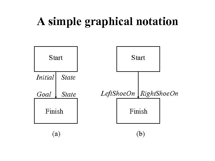 A simple graphical notation Start Initial State Goal State Start Left. Shoe. On Right. Shoe. On Finish (a) (b)
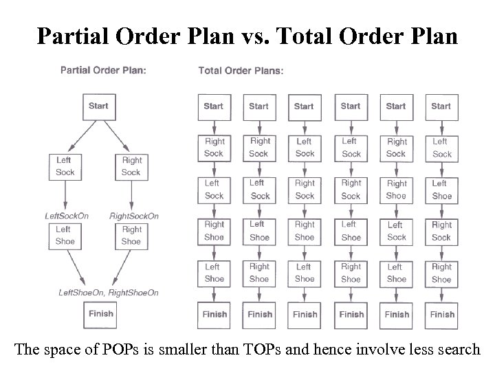 Partial Order Plan vs. Total Order Plan The space of POPs is smaller than TOPs and hence involve less search
 Least commitment • Non-linear planners embody the principle of least commitment – only choose actions, orderings, and variable bindings absolutely necessary, leaving other decisions till later – avoids early commitment to decisions that don’t really matter • A linear planner always chooses to add a plan step in a particular place in the sequence • A non-linear planner chooses to add a step and possibly some temporal constraints
 Non-linear plan • A non-linear plan consists of (1) A set of steps {S 1, S 2, S 3, S 4…} Steps have operator descriptions, preconditions & post-conditions (2) A set of causal links { … (Si, C, Sj) …} Purpose of step Si is to achieve precondition C of step Sj (3) A set of ordering constraints { … Si
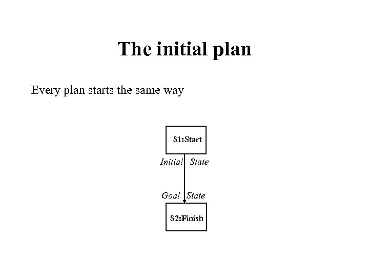 The initial plan Every plan starts the same way S 1: Start Initial State Goal State S 2: Finish
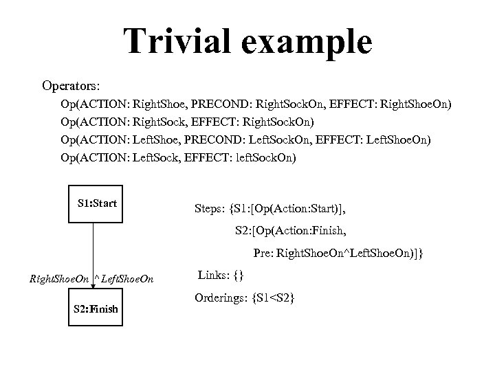 Trivial example Operators: Op(ACTION: Right. Shoe, PRECOND: Right. Sock. On, EFFECT: Right. Shoe. On) Op(ACTION: Right. Sock, EFFECT: Right. Sock. On) Op(ACTION: Left. Shoe, PRECOND: Left. Sock. On, EFFECT: Left. Shoe. On) Op(ACTION: Left. Sock, EFFECT: left. Sock. On) S 1: Start Steps: {S 1: [Op(Action: Start)], S 2: [Op(Action: Finish, Pre: Right. Shoe. On^Left. Shoe. On)]} Right. Shoe. On ^ Left. Shoe. On S 2: Finish Links: {} Orderings: {S 1
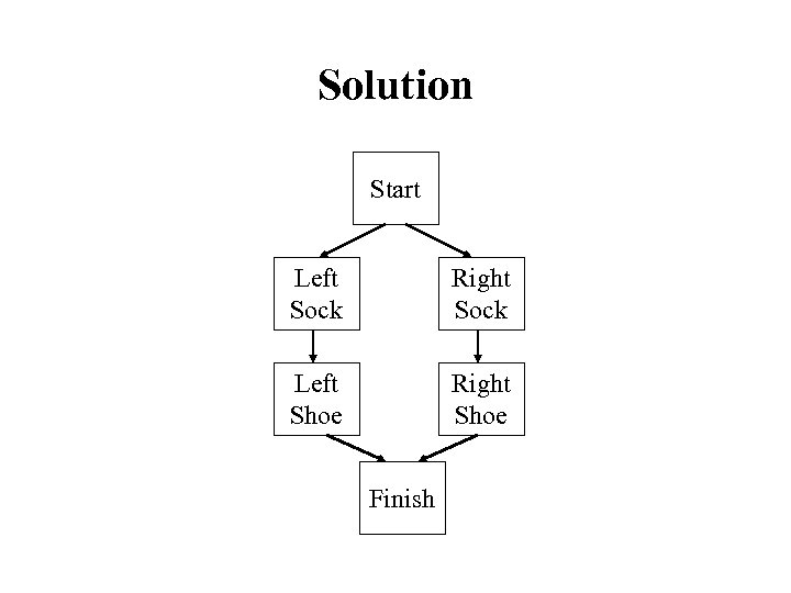 Solution Start Left Sock Right Sock Left Shoe Right Shoe Finish
 POP constraints and search heuristics • Only add steps that achieve a currently unachieved precondition • Use a least-commitment approach: – Don’t order steps unless they need to be ordered c • Honor causal links S 1 S 2 that protect condition c: – Never add an intervening step S 3 that violates c – If a parallel action threatens c (i. e. , has effect of negating or clobbering c), resolve threat by adding ordering links: • Order S 3 before S 1 (demotion) • Order S 3 after S 2 (promotion)
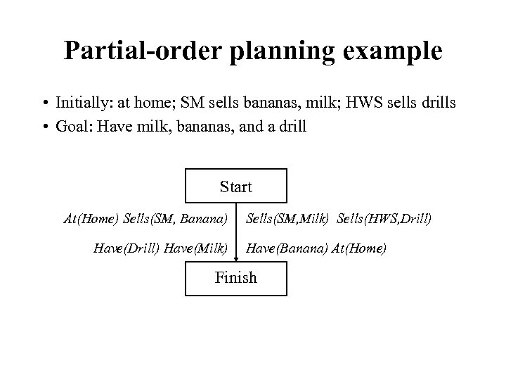 Partial-order planning example • Initially: at home; SM sells bananas, milk; HWS sells drills • Goal: Have milk, bananas, and a drill Start At(Home) Sells(SM, Banana) Have(Drill) Have(Milk) Sells(SM, Milk) Sells(HWS, Drill) Have(Banana) At(Home) Finish
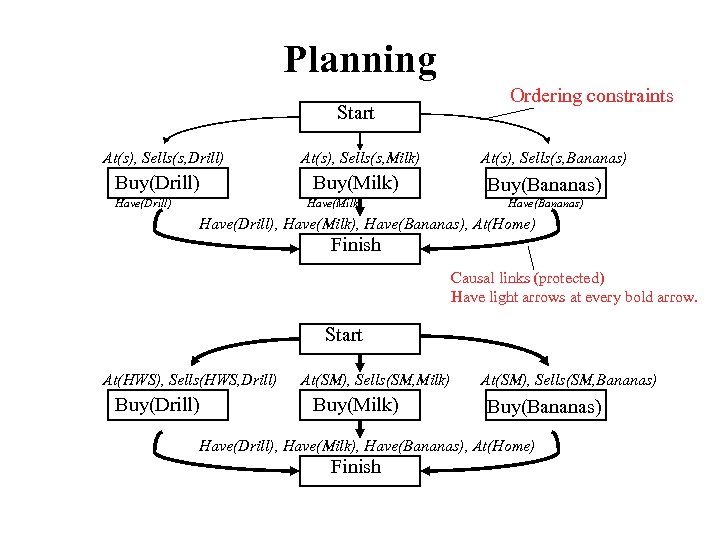 Planning Start At(s), Sells(s, Drill) Buy(Drill) Have(Drill) At(s), Sells(s, Milk) Buy(Milk) Have(Milk) Ordering constraints At(s), Sells(s, Bananas) Buy(Bananas) Have(Drill), Have(Milk), Have(Bananas), At(Home) Finish Causal links (protected) Have light arrows at every bold arrow. Start At(HWS), Sells(HWS, Drill) Buy(Drill) At(SM), Sells(SM, Milk) Buy(Milk) At(SM), Sells(SM, Bananas) Buy(Bananas) Have(Drill), Have(Milk), Have(Bananas), At(Home) Finish
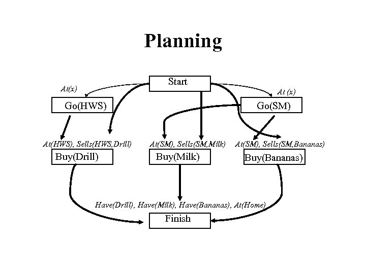 Planning Start At(x) At (x) Go(HWS) At(HWS), Sells(HWS, Drill) Buy(Drill) Go(SM) At(SM), Sells(SM, Milk) Buy(Milk) At(SM), Sells(SM, Bananas) Buy(Bananas) Have(Drill), Have(Milk), Have(Bananas), At(Home) Finish
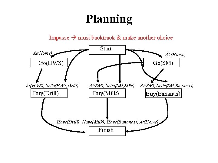 Planning Impasse must backtrack & make another choice Start At(Home) At (Home) Go(HWS) At(HWS), Sells(HWS, Drill) Buy(Drill) Go(SM) At(SM), Sells(SM, Milk) Buy(Milk) At(SM), Sells(SM, Bananas) Buy(Bananas) Have(Drill), Have(Milk), Have(Bananas), At(Home) Finish
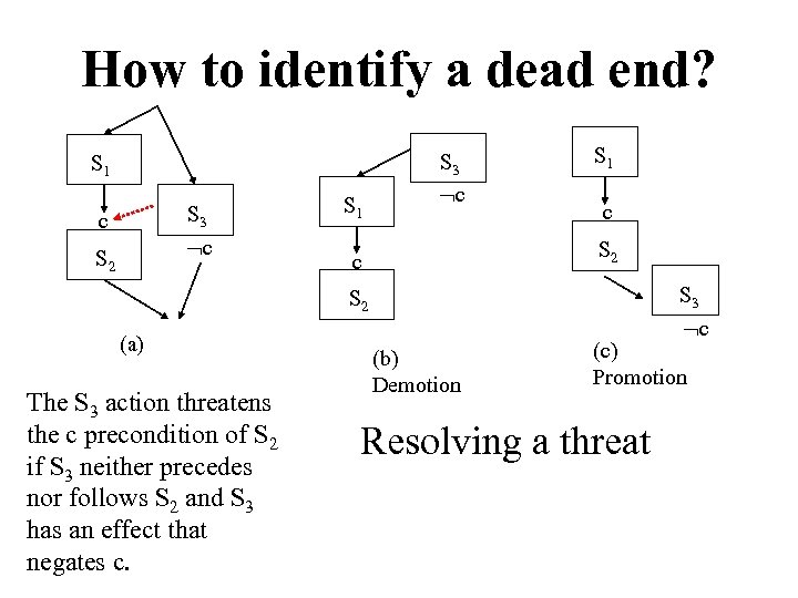 How to identify a dead end? S 1 S 3 c c S 2 S 1 S 3 c S 1 c S 2 c S 3 S 2 (a) The S 3 action threatens the c precondition of S 2 if S 3 neither precedes nor follows S 2 and S 3 has an effect that negates c. c (b) Demotion (c) Promotion Resolving a threat
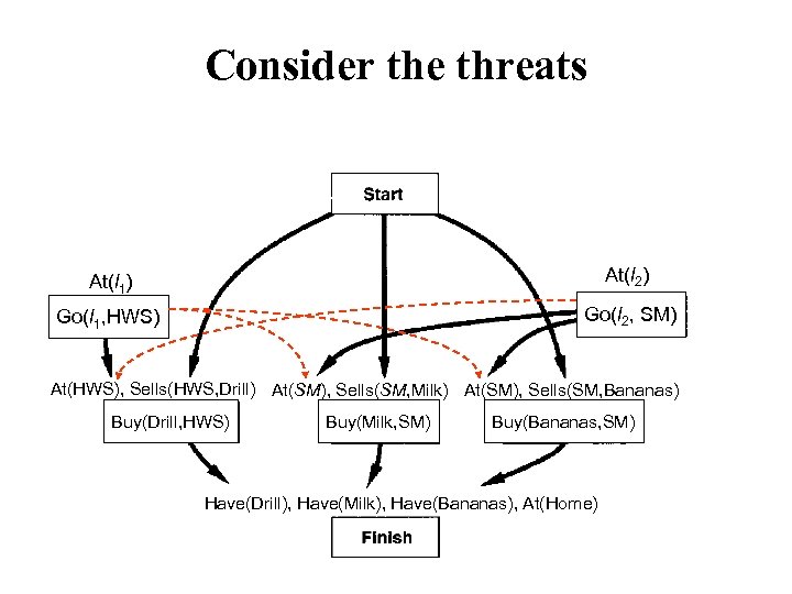 Consider the threats At(l 1) At(l At(x)2) Go(l 1, HWS) Go(l 2, SM) At(HWS), Sells(HWS, Drill) At(SM), Sells(SM, Milk) At(SM), Sells(SM, Bananas) Buy(Drill, HWS) Buy(Milk, SM) Buy(Bananas, SM) Have(Drill), Have(Milk), Have(Bananas), At(Home)
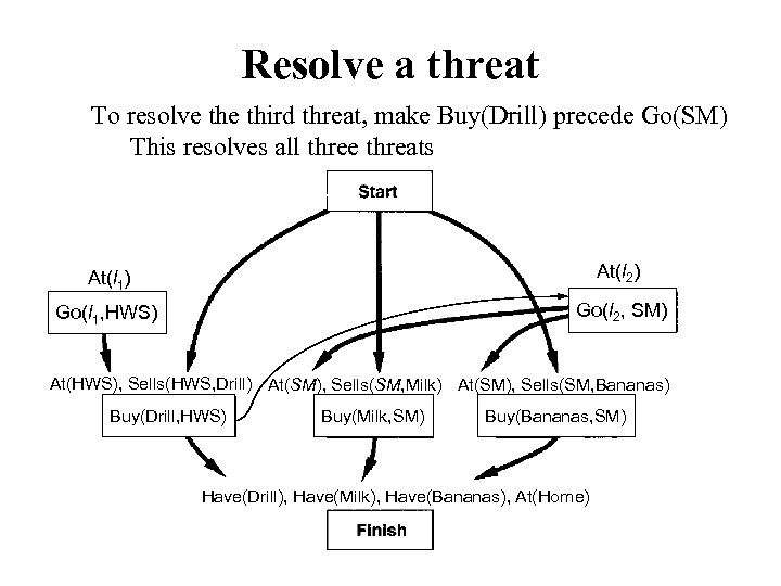 Resolve a threat To resolve third threat, make Buy(Drill) precede Go(SM) This resolves all three threats • To resolve third threat, make Buy(Drill) precede Go(SM) – This resolves all three threats At(l 1) At(l At(x)2) Go(l 1, HWS) Go(l 2, SM) At(HWS), Sells(HWS, Drill) At(SM), Sells(SM, Milk) At(SM), Sells(SM, Bananas) Buy(Drill, HWS) Buy(Milk, SM) Buy(Bananas, SM) Have(Drill), Have(Milk), Have(Bananas), At(Home)
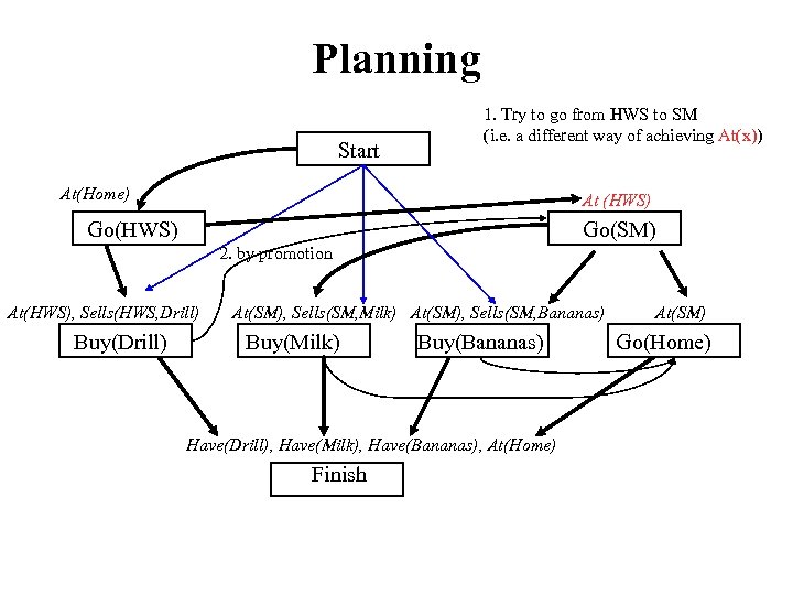 Planning Start 1. Try to go from HWS to SM (i. e. a different way of achieving At(x)) At(Home) At (HWS) Go(SM) 2. by promotion At(HWS), Sells(HWS, Drill) Buy(Drill) At(SM), Sells(SM, Milk) At(SM), Sells(SM, Bananas) Buy(Milk) Buy(Bananas) Have(Drill), Have(Milk), Have(Bananas), At(Home) Finish At(SM) Go(Home)
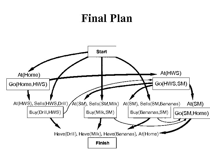 Final Plan • Establish At(l 3) with l 3=SM At(Home) At(HWS) At(x) Go(Home, HWS) Go(HWS, SM) At(HWS), Sells(HWS, Drill) At(SM), Sells(SM, Milk) At(SM), Sells(SM, Bananas) Buy(Drill, HWS) Buy(Milk, SM) Buy(Bananas, SM) Have(Drill), Have(Milk), Have(Bananas), At(Home) At(SM) Go(SM, Home)
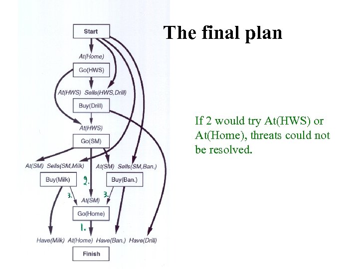 The final plan If 2 would try At(HWS) or At(Home), threats could not be resolved.
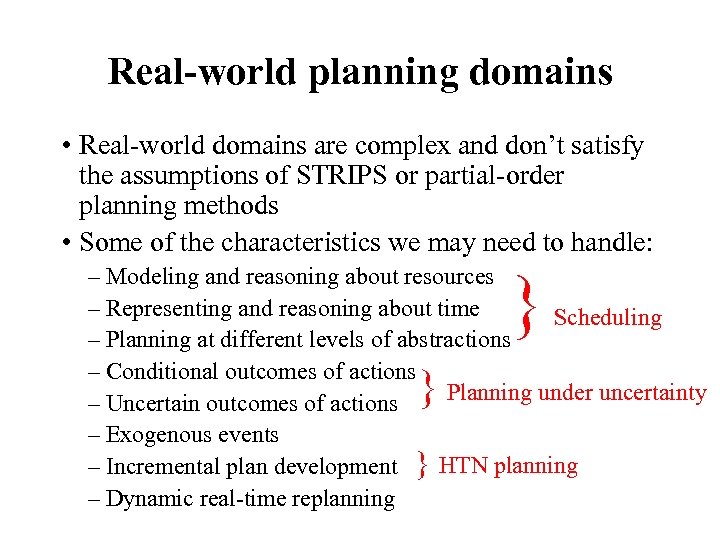 Real-world planning domains • Real-world domains are complex and don’t satisfy the assumptions of STRIPS or partial-order planning methods • Some of the characteristics we may need to handle: } – Modeling and reasoning about resources – Representing and reasoning about time Scheduling – Planning at different levels of abstractions – Conditional outcomes of actions Planning under uncertainty – Uncertain outcomes of actions – Exogenous events – Incremental plan development } HTN planning – Dynamic real-time replanning }
 Hierarchical decomposition • Hierarchical decomposition, or hierarchical task network (HTN) planning, uses abstract operators to incrementally decompose a planning problem from a high-level goal statement to a primitive plan network • Primitive operators represent actions that are executable, and can appear in the final plan • Non-primitive operators represent goals (equivalently, abstract actions) that require further decomposition (or operationalization) to be executed • There is no “right” set of primitive actions: One agent’s goals are another agent’s actions!
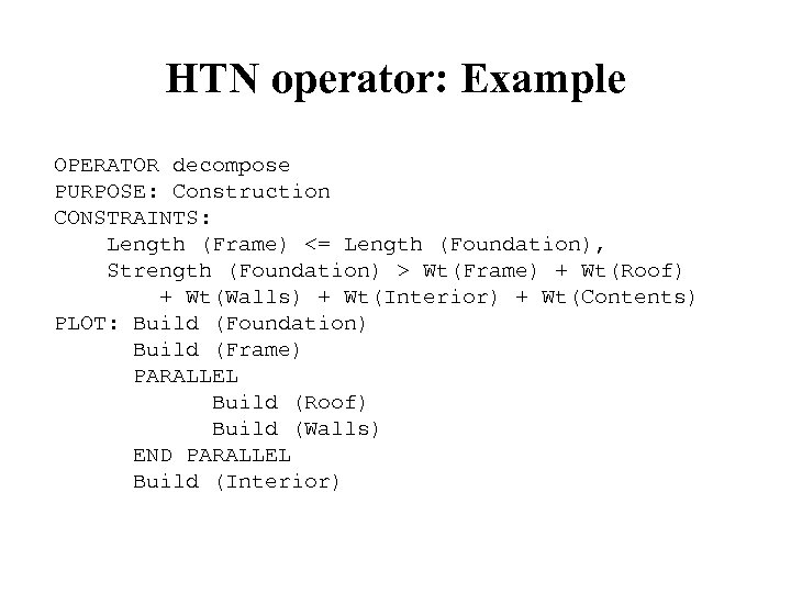 HTN operator: Example OPERATOR decompose PURPOSE: Construction CONSTRAINTS: Length (Frame) <= Length (Foundation), Strength (Foundation) > Wt(Frame) + Wt(Roof) + Wt(Walls) + Wt(Interior) + Wt(Contents) PLOT: Build (Foundation) Build (Frame) PARALLEL Build (Roof) Build (Walls) END PARALLEL Build (Interior)
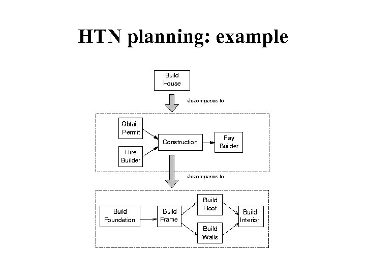 HTN planning: example
 HTN operator representation • Russell & Norvig explicitly represent causal links; these can also be computed dynamically by using a model of preconditions and effects • Dynamically computing causal links means that actions from one operator can safely be interleaved with other operators, and subactions can safely be removed or replaced during plan repair • Russell & Norvig’s representation only includes variable bindings, but more generally we can introduce a wide array of variable constraints
 Truth criterion • Determining if a formula is true at a particular point in a partially ordered plan is, in general, NP-hard • Intuition: there are exponentially many ways to linearize a partially ordered plan • Worst case: if there are N actions unordered with respect to each other, there are N! linearizations • Ensuring soundness of truth criterion requires checking formula under all possible linearizations • Use heuristic methods instead to make planning feasible • Check later to ensure no constraints are violated
 Truth criterion in HTN planners • Heuristic: prove that there is one possible ordering of the actions that makes the formula true – but don’t insert ordering links to enforce that order • Such a proof is efficient – Suppose you have an action A 1 with a precondition P – Find an action A 2 that achieves P (A 2 could be initial world state) – Make sure there is no action necessarily between A 2 and A 1 that negates P • Applying this heuristic for all preconditions in the plan can result in infeasible plans
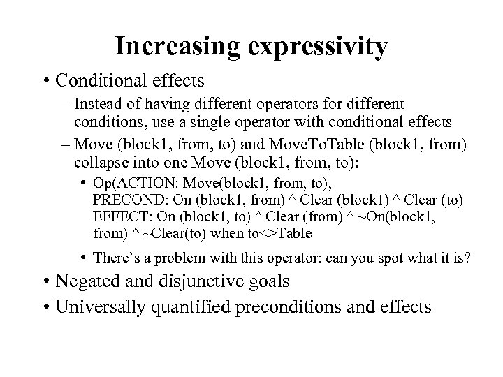 Increasing expressivity • Conditional effects – Instead of having different operators for different conditions, use a single operator with conditional effects – Move (block 1, from, to) and Move. To. Table (block 1, from) collapse into one Move (block 1, from, to): • Op(ACTION: Move(block 1, from, to), PRECOND: On (block 1, from) ^ Clear (block 1) ^ Clear (to) EFFECT: On (block 1, to) ^ Clear (from) ^ ~On(block 1, from) ^ ~Clear(to) when to<>Table • There’s a problem with this operator: can you spot what it is? • Negated and disjunctive goals • Universally quantified preconditions and effects
 Reasoning about resources • Introduce numeric variables used as measures • These variables represent resource quantities, and change over the course of the plan • Certain actions may produce (increase the quantity of) resources • Other actions may consume (decrease the quantity of) resources • More generally, may want different resource types – Continuous vs. discrete – Sharable vs. nonsharable – Reusable vs. consumable vs. self-replenishing
 Other real-world planning issues • Conditional planning • Partial observability • Information gathering actions • Execution monitoring and replanning • Continuous planning • Multi-agent (cooperative or adversarial) planning
 Planning summary • Planning representations – Situation calculus – STRIPS representation: Preconditions and effects • Planning approaches – State-space search (STRIPS, forward chaining, …. ) – Plan-space search (partial-order planning, HTN, …) – Constraint-based search (Graph. Plan, SATplan, …) • Search strategies – – – Forward planning Goal regression Backward planning Least-commitment Nonlinear planning


