Plan q Dynamic programming q Introduction to Markov

Plan q. Dynamic programming q. Introduction to Markov decision processes q. Markov decision processes formulation q. Discounted markov decision processes q. Average cost markov decision processes q. Continuous-time Markov decision processes Xiaolan Xie

Dynamic programming q. Basic principe of dynamic programming q. Some applications q. Stochastic dynamic programming Xiaolan Xie

Dynamic programming q. Basic principe of dynamic programming q. Some applications q. Stochastic dynamic programming Xiaolan Xie

Introduction q. Dynamic programming (DP) is a general optimization technique based on implicit enumeration of the solution space. q. The problems should have a particular sequential structure, such that the set of unknowns can be made sequentially. q. It is based on the "principle of optimality" q. A wide range of problems can be put in seqential form and solved by dynamic programming Xiaolan Xie

Introduction Applications : • Optimal control • Most problems in graph theory • Investment • Deterministic and stochastic inventory control • Project scheduling • Production scheduling We limit ourselves to discrete optimization Xiaolan Xie

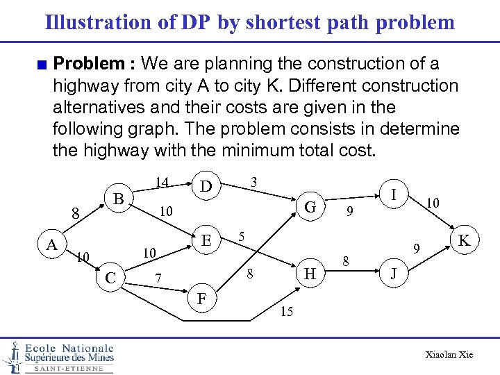Illustration of DP by shortest path problem Problem : We are planning the construction of a highway from city A to city K. Different construction alternatives and their costs are given in the following graph. The problem consists in determine the highway with the minimum total cost. 8 A B 14 C G 10 10 10 3 D E H F 10 9 5 8 7 I 8 9 K J 15 Xiaolan Xie

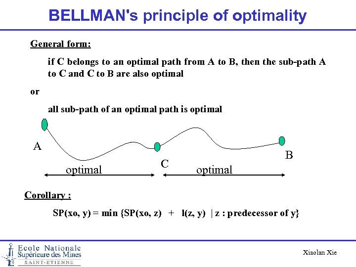BELLMAN's principle of optimality General form: if C belongs to an optimal path from A to B, then the sub-path A to C and C to B are also optimal or all sub-path of an optimal path is optimal A optimal C B optimal Corollary : SP(xo, y) = min {SP(xo, z) + l(z, y) | z : predecessor of y} Xiaolan Xie

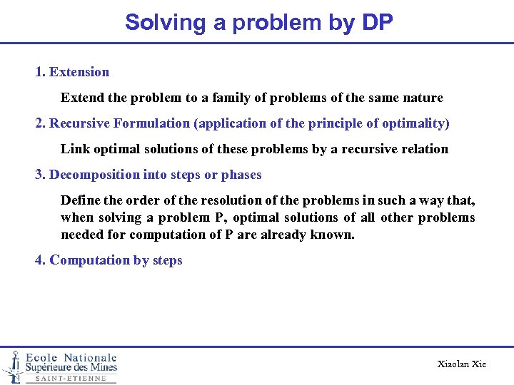Solving a problem by DP 1. Extension Extend the problem to a family of problems of the same nature 2. Recursive Formulation (application of the principle of optimality) Link optimal solutions of these problems by a recursive relation 3. Decomposition into steps or phases Define the order of the resolution of the problems in such a way that, when solving a problem P, optimal solutions of all other problems needed for computation of P are already known. 4. Computation by steps Xiaolan Xie

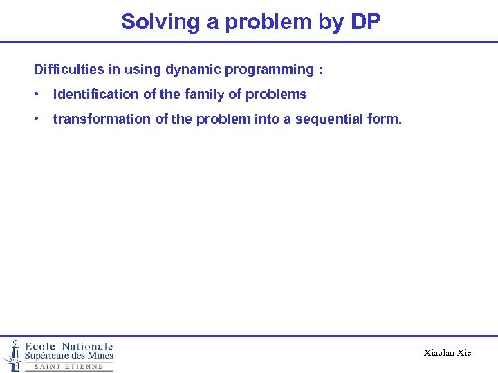Solving a problem by DP Difficulties in using dynamic programming : • Identification of the family of problems • transformation of the problem into a sequential form. Xiaolan Xie

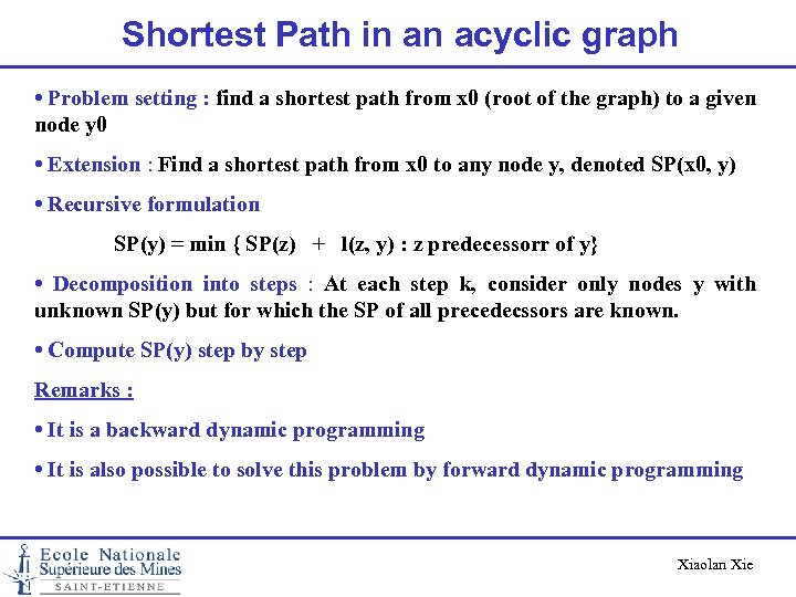Shortest Path in an acyclic graph • Problem setting : find a shortest path from x 0 (root of the graph) to a given node y 0 • Extension : Find a shortest path from x 0 to any node y, denoted SP(x 0, y) • Recursive formulation SP(y) = min { SP(z) + l(z, y) : z predecessorr of y} • Decomposition into steps : At each step k, consider only nodes y with unknown SP(y) but for which the SP of all precedecssors are known. • Compute SP(y) step by step Remarks : • It is a backward dynamic programming • It is also possible to solve this problem by forward dynamic programming Xiaolan Xie

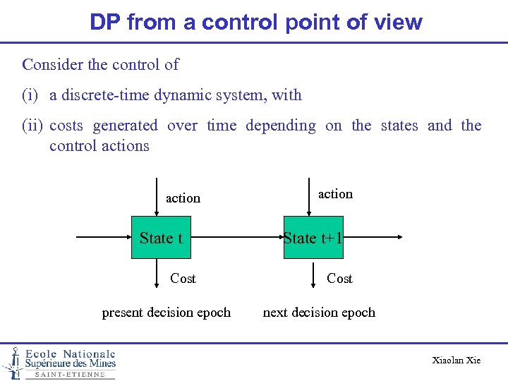DP from a control point of view Consider the control of (i) a discrete-time dynamic system, with (ii) costs generated over time depending on the states and the control actions action State t Cost present decision epoch action State t+1 Cost next decision epoch Xiaolan Xie

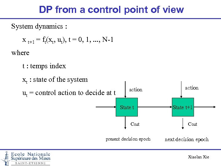DP from a control point of view System dynamics : x t+1 = ft(xt, ut), t = 0, 1, . . . , N-1 where t : temps index xt : state of the system ut = control action to decide at t action State t Cost present decision epoch action State t+1 Cost next decision epoch Xiaolan Xie

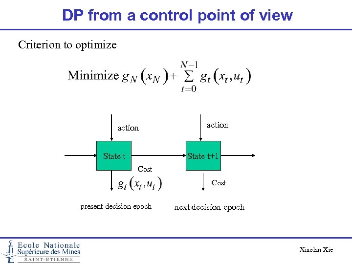DP from a control point of view Criterion to optimize action State t+1 Cost present decision epoch next decision epoch Xiaolan Xie

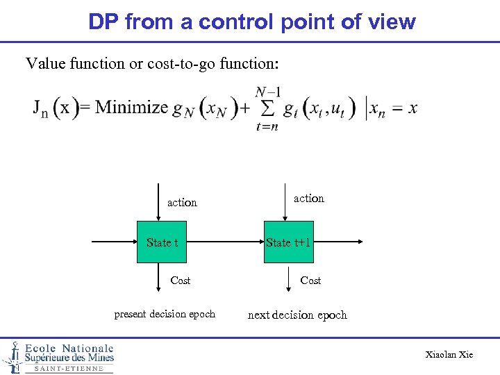DP from a control point of view Value function or cost-to-go function: action State t Cost present decision epoch action State t+1 Cost next decision epoch Xiaolan Xie

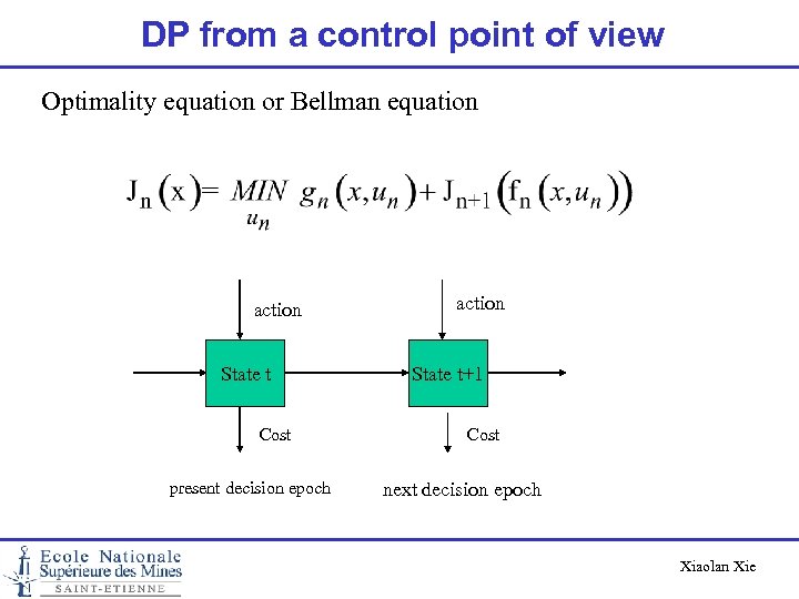DP from a control point of view Optimality equation or Bellman equation action State t Cost present decision epoch action State t+1 Cost next decision epoch Xiaolan Xie

Applications Single machine scheduling (Knapsac) Inventory control Traveling salesman problem Xiaolan Xie

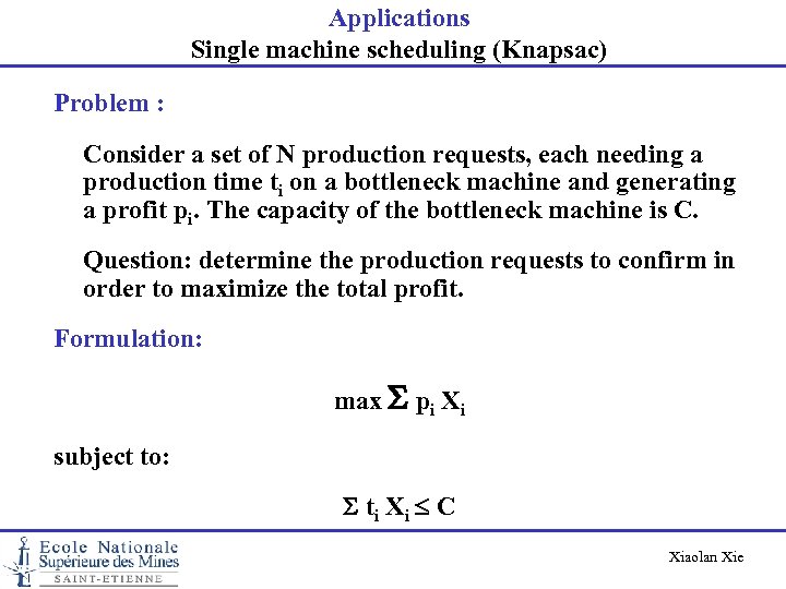Applications Single machine scheduling (Knapsac) Problem : Consider a set of N production requests, each needing a production time ti on a bottleneck machine and generating a profit pi. The capacity of the bottleneck machine is C. Question: determine the production requests to confirm in order to maximize the total profit. Formulation: max pi Xi subject to: ti Xi C Xiaolan Xie

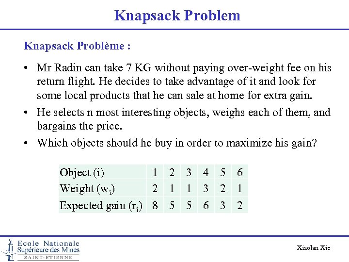Knapsack Problem Knapsack Problème : • Mr Radin can take 7 KG without paying over-weight fee on his return flight. He decides to take advantage of it and look for some local products that he can sale at home for extra gain. • He selects n most interesting objects, weighs each of them, and bargains the price. • Which objects should he buy in order to maximize his gain? Object (i) 1 2 3 4 5 6 Weight (wi) 2 1 1 3 2 1 Expected gain (ri) 8 5 5 6 3 2 Xiaolan Xie

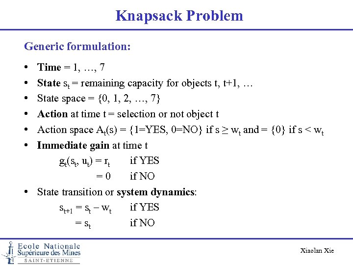Knapsack Problem Generic formulation: • • • Time = 1, …, 7 State st = remaining capacity for objects t, t+1, … State space = {0, 1, 2, …, 7} Action at time t = selection or not object t Action space At(s) = {1=YES, 0=NO} if s ≥ wt and = {0} if s < wt Immediate gain at time t gt(st, ut) = rt if YES = 0 if NO • State transition or system dynamics: st+1 = st – wt if YES = st if NO Xiaolan Xie

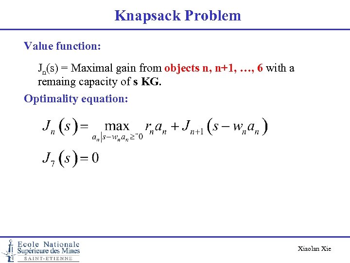Knapsack Problem Value function: Jn(s) = Maximal gain from objects n, n+1, …, 6 with a remaing capacity of s KG. Optimality equation: Xiaolan Xie

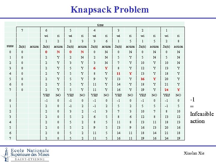Knapsack Problem time state 0 1 2 3 4 5 6 7 7 Jn(s) 0 0 0 0 action 6 wi 1 Jn(s) 0 2 2 2 2 YES -1 2 2 2 2 ri 2 action N Y Y Y Y NO 0 0 0 0 5 wi 2 Jn(s) 0 2 3 5 5 5 YES -1 -1 3 5 5 5 ri 3 action N N Y Y Y NO 0 2 2 2 2 4 wi 3 Jn(s) 0 2 3 6 8 9 11 11 YES -1 -1 -1 6 8 9 11 11 ri 6 action N N N Y Y Y NO 0 2 3 5 5 5 3 wi 1 Jn(s) 0 5 7 8 11 13 14 16 YES -1 5 7 8 11 13 14 16 ri 5 action N Y Y Y Y NO 0 2 3 6 8 9 11 11 2 wi 1 Jn(s) 0 5 10 12 13 16 18 19 YES -1 5 10 12 13 16 18 19 ri 5 action N N Y Y Y NO 0 5 7 8 11 13 14 16 1 wi 2 Jn(s) 0 5 10 13 18 20 21 24 YES -1 -1 8 13 18 20 21 24 ri 8 action N N N Y Y Y NO 0 5 10 12 13 16 18 19 -1 = Infeasible action Xiaolan Xie

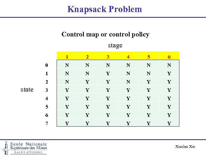Knapsack Problem Control map or control policy stage 1 3 4 5 6 0 N N N 1 N N Y 2 state 2 N Y Y 3 Y Y Y 4 Y Y Y 5 Y Y Y 6 Y Y Y 7 Y Y Y Xiaolan Xie

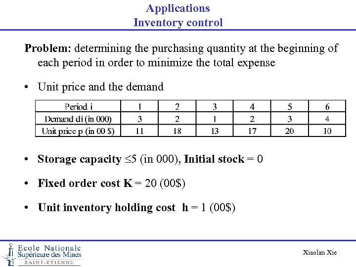Applications Inventory control Problem: determining the purchasing quantity at the beginning of each period in order to minimize the total expense • Unit price and the demand • Storage capacity 5 (in 000), Initial stock = 0 • Fixed order cost K = 20 (00$) • Unit inventory holding cost h = 1 (00$) Xiaolan Xie

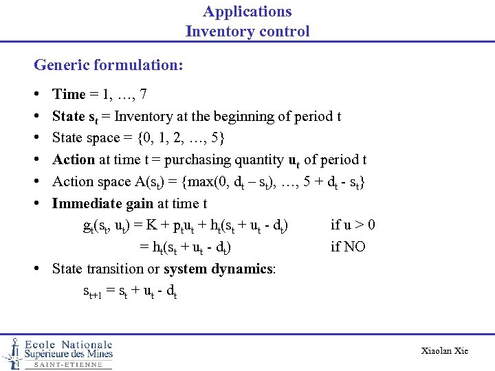Applications Inventory control Generic formulation: • • • Time = 1, …, 7 State st = Inventory at the beginning of period t State space = {0, 1, 2, …, 5} Action at time t = purchasing quantity ut of period t Action space A(st) = {max(0, dt – st), …, 5 + dt - st} Immediate gain at time t gt(st, ut) = K + ptut + ht(st + ut - dt) if u > 0 = ht(st + ut - dt) if NO • State transition or system dynamics: st+1 = st + ut - dt Xiaolan Xie

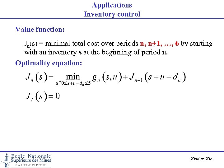Applications Inventory control Value function: Jn(s) = minimal total cost over periods n, n+1, …, 6 by starting with an inventory s at the beginning of period n. Optimality equation: Xiaolan Xie

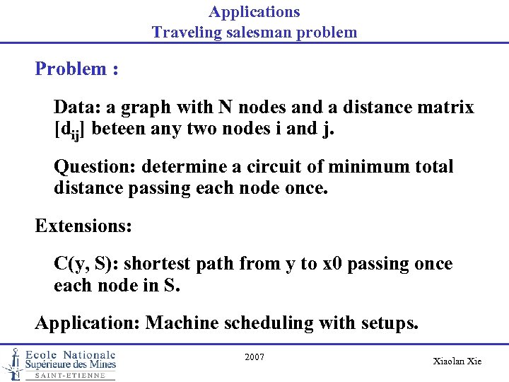Applications Traveling salesman problem Problem : Data: a graph with N nodes and a distance matrix [dij] beteen any two nodes i and j. Question: determine a circuit of minimum total distance passing each node once. Extensions: C(y, S): shortest path from y to x 0 passing once each node in S. Application: Machine scheduling with setups. 2007 Xiaolan Xie

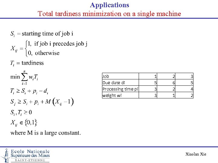Applications Total tardiness minimization on a single machine Job Due date di Processing time pi weight wi 1 5 3 3 2 6 2 1 3 5 4 2 Xiaolan Xie

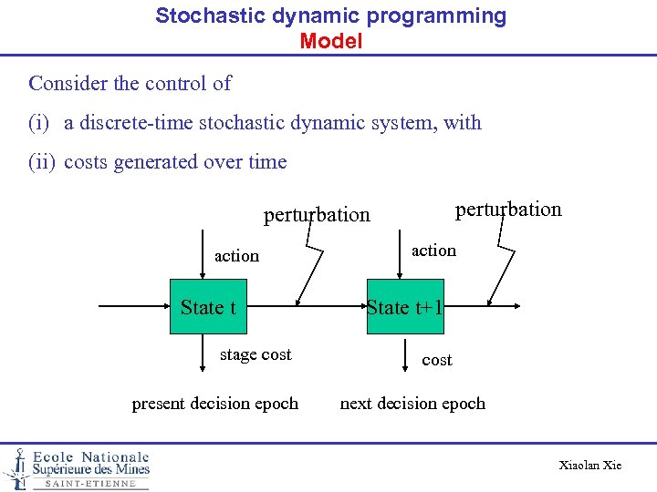Stochastic dynamic programming Model Consider the control of (i) a discrete-time stochastic dynamic system, with (ii) costs generated over time perturbation action State t stage cost present decision epoch action State t+1 cost next decision epoch Xiaolan Xie

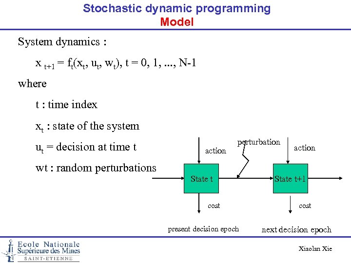Stochastic dynamic programming Model System dynamics : x t+1 = ft(xt, ut, wt), t = 0, 1, . . . , N-1 where t : time index xt : state of the system ut = decision at time t wt : random perturbations action perturbation State t cost present decision epoch action State t+1 cost next decision epoch Xiaolan Xie

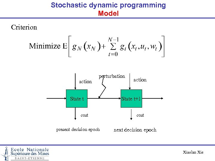Stochastic dynamic programming Model Criterion action perturbation State t cost present decision epoch action State t+1 cost next decision epoch Xiaolan Xie

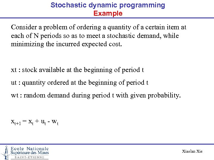Stochastic dynamic programming Example Consider a problem of ordering a quantity of a certain item at each of N periods so as to meet a stochastic demand, while minimizing the incurred expected cost. xt : stock available at the beginning of period t ut : quantity ordered at the beginning of period t wt : random demand during period t with given probability. xt+1 = xt + ut - wt Xiaolan Xie

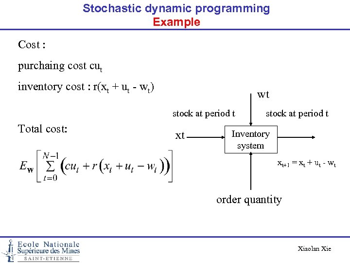Stochastic dynamic programming Example Cost : purchaing cost cut inventory cost : r(xt + ut - wt) wt stock at period t Total cost: xt stock at period t Inventory system xt+1 = xt + ut - wt order quantity Xiaolan Xie

Stochastic dynamic programming Model Open-loop control: Order quantities u 1, u 2, . . . , u. N-1 are determined once at time 0 Closed-loop control: Order quantity ut at each period is determined dynamically with the knowledge of state xt Xiaolan Xie

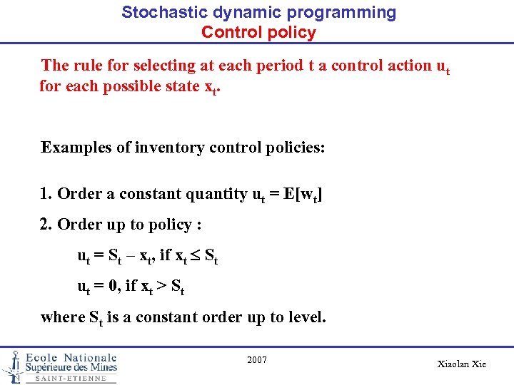Stochastic dynamic programming Control policy The rule for selecting at each period t a control action ut for each possible state xt. Examples of inventory control policies: 1. Order a constant quantity ut = E[wt] 2. Order up to policy : ut = St – xt, if xt St ut = 0, if xt > St where St is a constant order up to level. 2007 Xiaolan Xie

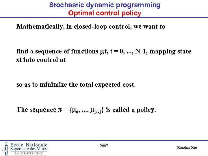Stochastic dynamic programming Optimal control policy Mathematically, in closed-loop control, we want to find a sequence of functions mt, t = 0, . . . , N-1, mapping state xt into control ut so as to minimize the total expected cost. The sequence p = {m 0, . . . , m. N-1} is called a policy. 2007 Xiaolan Xie

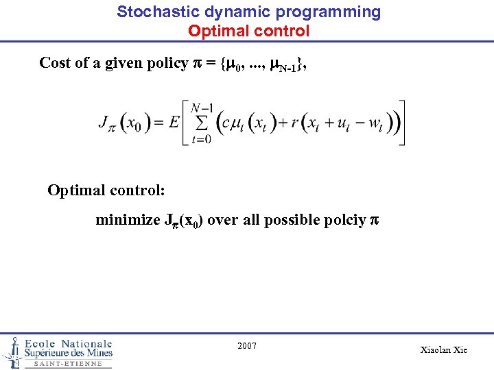Stochastic dynamic programming Optimal control Cost of a given policy p = {m 0, . . . , m. N-1}, Optimal control: minimize Jp(x 0) over all possible polciy p 2007 Xiaolan Xie

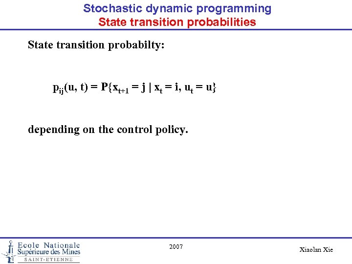Stochastic dynamic programming State transition probabilities State transition probabilty: pij(u, t) = P{xt+1 = j | xt = i, ut = u} depending on the control policy. 2007 Xiaolan Xie

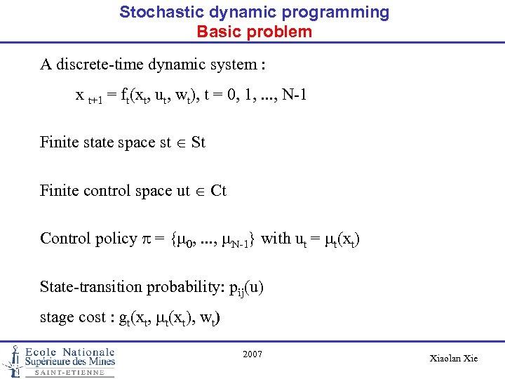Stochastic dynamic programming Basic problem A discrete-time dynamic system : x t+1 = ft(xt, ut, wt), t = 0, 1, . . . , N-1 Finite state space st St Finite control space ut Ct Control policy p = {m 0, . . . , m. N-1} with ut = mt(xt) State-transition probability: pij(u) stage cost : gt(xt, mt(xt), wt) 2007 Xiaolan Xie

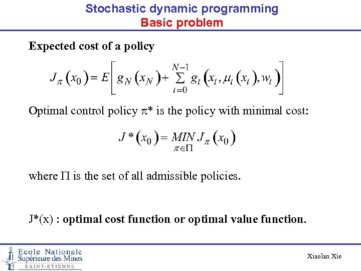Stochastic dynamic programming Basic problem Expected cost of a policy Optimal control policy p* is the policy with minimal cost: where P is the set of all admissible policies. J*(x) : optimal cost function or optimal value function. Xiaolan Xie

Stochastic dynamic programming Principle of optimality Let p* = {m*0, . . . , m*N-1} be an optimal policy for the basic problem for the N time periods. Then the truncated policy {m*i, . . . , m*N-1} is optimal for the following subproblem • minimization of the following total cost (called cost-to-go function) from time i to time N by starting with state xi at time i Xiaolan Xie

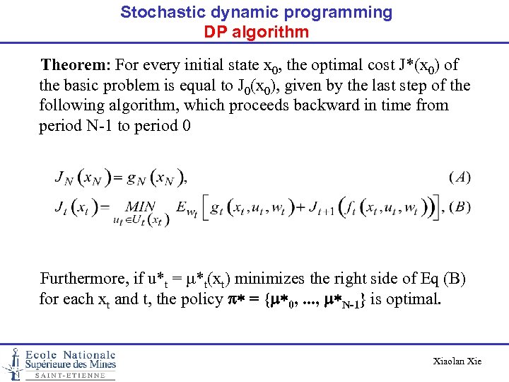Stochastic dynamic programming DP algorithm Theorem: For every initial state x 0, the optimal cost J*(x 0) of the basic problem is equal to J 0(x 0), given by the last step of the following algorithm, which proceeds backward in time from period N-1 to period 0 Furthermore, if u*t = m*t(xt) minimizes the right side of Eq (B) for each xt and t, the policy p* = {m*0, . . . , m*N-1} is optimal. Xiaolan Xie

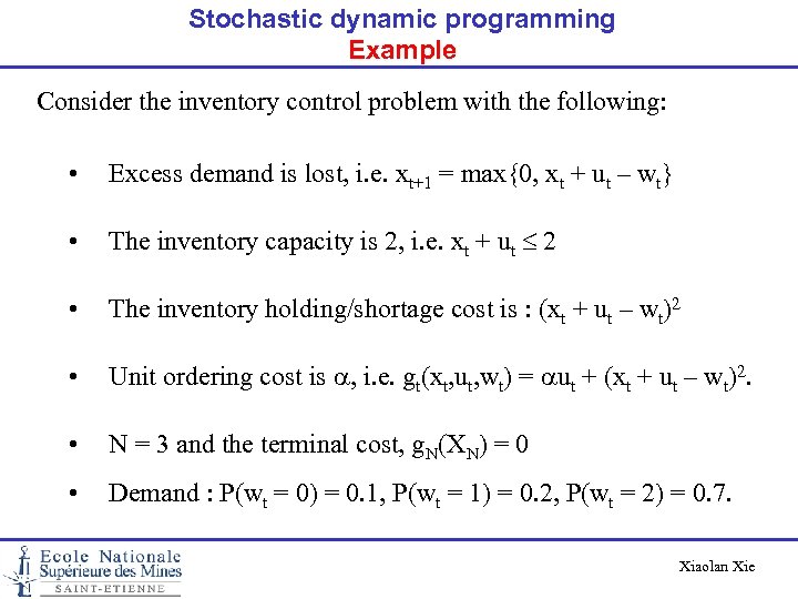Stochastic dynamic programming Example Consider the inventory control problem with the following: • Excess demand is lost, i. e. xt+1 = max{0, xt + ut – wt} • The inventory capacity is 2, i. e. xt + ut 2 • The inventory holding/shortage cost is : (xt + ut – wt)2 • Unit ordering cost is a, i. e. gt(xt, ut, wt) = aut + (xt + ut – wt)2. • N = 3 and the terminal cost, g. N(XN) = 0 • Demand : P(wt = 0) = 0. 1, P(wt = 1) = 0. 2, P(wt = 2) = 0. 7. Xiaolan Xie

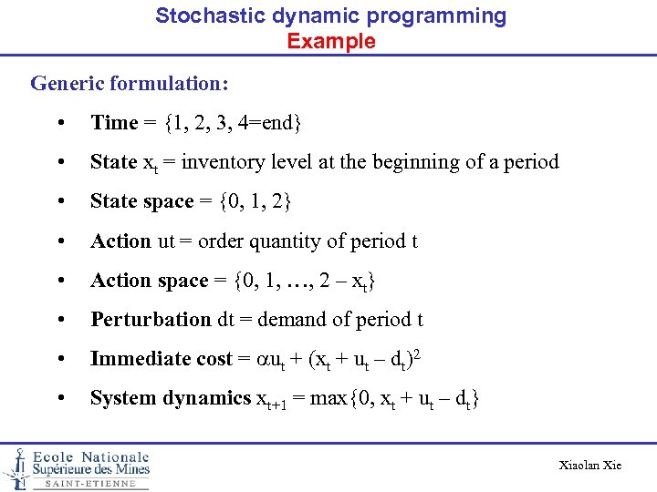Stochastic dynamic programming Example Generic formulation: • Time = {1, 2, 3, 4=end} • State xt = inventory level at the beginning of a period • State space = {0, 1, 2} • Action ut = order quantity of period t • Action space = {0, 1, …, 2 – xt} • Perturbation dt = demand of period t • Immediate cost = aut + (xt + ut – dt)2 • System dynamics xt+1 = max{0, xt + ut – dt} Xiaolan Xie

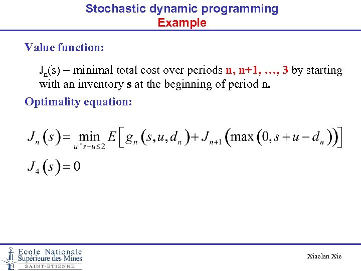Stochastic dynamic programming Example Value function: Jn(s) = minimal total cost over periods n, n+1, …, 3 by starting with an inventory s at the beginning of period n. Optimality equation: Xiaolan Xie

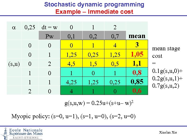Stochastic dynamic programming Example – Immediate cost a 0, 25 dt = w Pw 0 0 0 1 (s, u) 0 2 1 0 1 1 2 0 0 0, 1 0 1, 25 4, 5 1 4, 25 4 1 0, 25 1, 5 0 1, 25 1 2 0, 7 4 1, 25 0, 5 1 0, 25 0 mean 3 1, 05 1, 1 0, 85 0, 6 mean stage cost = 0. 1 g(s, u, 0)+ 0. 2 g(s, u, 1)+ 0. 7 g(s, u, 2) g(s, u, w) = 0. 25 u+(s+u– w)2 Myopic policy: (s=0, u=1), (s=1, u=0), (s=2, u=0) Xiaolan Xie

Stochastic dynamic programming Example – Period 3 -problem Period n = 3 a 0, 25 dt = w 0 1 2 Mean Pw 0, 1 0, 2 0, 7 0 0 0 1 4 0 1 1, 25 0, 25 1, 25 0 2 4, 5 1, 5 0, 5 total 3 1, 05 1, 1 0, 85 0, 6 period-4 opt s' J 4(s') (s, u) 0 0 1 0 1 1 4, 25 1, 25 0, 25 2 0 4 1 0 Stage cost 0. 25 u+(s+u– w)2 + Remaining cost J 4((s+u-w)+) Xiaolan Xie

Stochastic dynamic programming Example – Periods 2+3 -problem a period-3 opt s' (s, u) J 3(s') 0 1, 05 1 0, 8 2 0, 6 0, 25 0 0 0 1 1 2 Period n = 2 dt = w 0 Pw 0, 1 0 1, 05 1 2, 05 2 5, 1 0 1, 8 1 4, 85 0 4, 6 1 0, 2 2, 05 1, 3 2, 3 1, 05 2, 05 1, 8 2 0, 7 5, 05 2, 3 1, 55 2, 05 1, 3 1, 05 Mean total 4, 05 2, 075 2, 055 1, 825 1, 805 1, 555 Xiaolan Xie

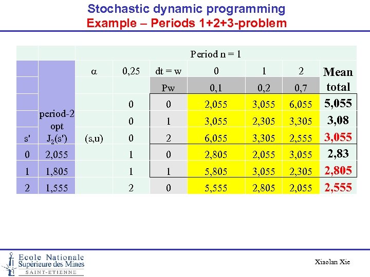Stochastic dynamic programming Example – Periods 1+2+3 -problem Period n = 1 a 0, 25 dt = w 0 1 2 Pw 0, 1 0, 2 0, 7 0 0 2, 055 3, 055 6, 055 0 1 3, 055 2, 305 3, 305 0 2 6, 055 3, 305 2, 555 period-2 opt s' (s, u) J 2(s') 0 2, 055 1 0 2, 805 2, 055 3, 055 1 1, 805 1 1 5, 805 3, 055 2, 305 2 1, 555 2 0 5, 555 2, 805 2, 055 Mean total 5, 055 3, 08 3, 055 2, 83 2, 805 2, 555 Xiaolan Xie

Stochastic dynamic programming Example – value function & control Optimal policy a =0, 25 Stock 3 -period policy 2 -period policy 1 -period policy Stage 1 Stage 2 Stage 3 Cos-to-go (order quantity) 0 3. 055 (2) 2. 055 (2) 1. 05 (1) 1 2. 805 (1) 1. 805 (1) 0. 8 (0) 2 2. 555 (0) 1. 555 (0) 0. 6 (0) Xiaolan Xie

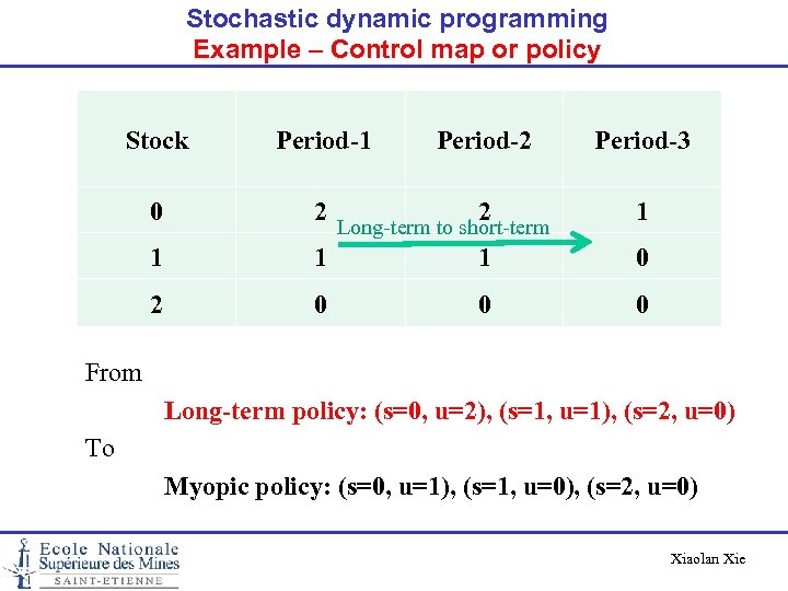Stochastic dynamic programming Example – Control map or policy Stock Period-1 Period-2 Period-3 0 2 2 1 1 0 2 0 0 0 Long-term to short-term From Long-term policy: (s=0, u=2), (s=1, u=1), (s=2, u=0) To Myopic policy: (s=0, u=1), (s=1, u=0), (s=2, u=0) Xiaolan Xie

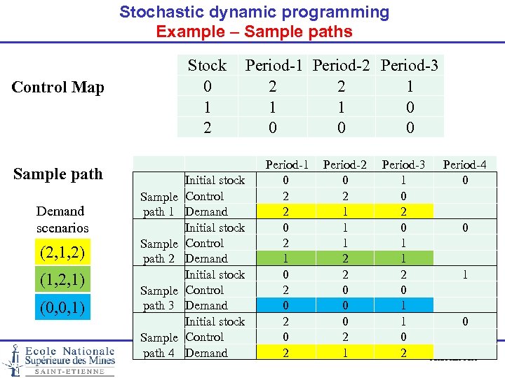Stochastic dynamic programming Example – Sample paths Stock Period-1 Period-2 Period-3 0 2 2 1 1 0 2 0 0 0 Control Map Sample path Demand scenarios (2, 1, 2) (1, 2, 1) (0, 0, 1) Sample path 1 Sample path 2 Sample path 3 Sample path 4 Initial stock Control Demand Period-1 0 2 2 0 2 1 0 2 0 2 Period-2 0 2 1 1 1 2 2 0 0 0 2 1 Period-3 1 0 2 0 1 1 0 2 Period-4 0 0 1 0 Xiaolan Xie

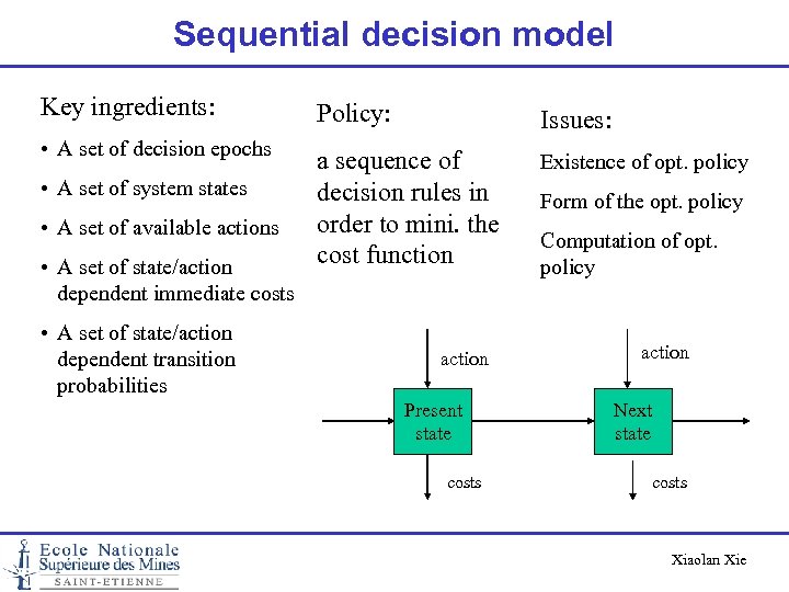Sequential decision model Key ingredients: Policy: Issues: • A set of decision epochs a sequence of decision rules in order to mini. the cost function Existence of opt. policy • A set of system states • A set of available actions • A set of state/action dependent immediate costs • A set of state/action dependent transition probabilities action Present state costs Form of the opt. policy Computation of opt. policy action Next state costs Xiaolan Xie

Applications Inventory management Bus engine replacement Highway pavement maintenance Bed allocation in hospitals Personal staffing in fire department Traffic control in communication networks … Xiaolan Xie

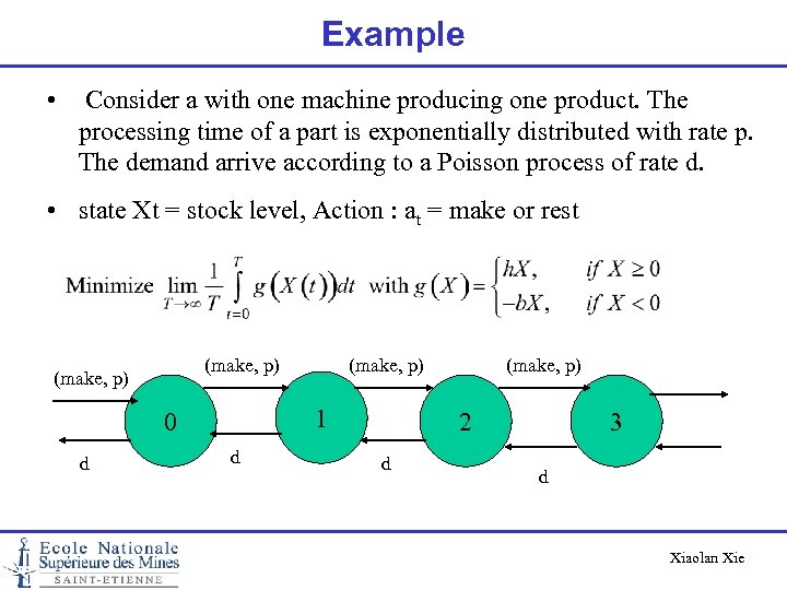Example • Consider a with one machine producing one product. The processing time of a part is exponentially distributed with rate p. The demand arrive according to a Poisson process of rate d. • state Xt = stock level, Action : at = make or rest (make, p) 1 0 d (make, p) 2 d 3 d Xiaolan Xie

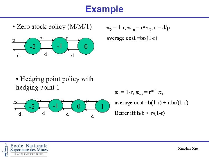Example • Zero stock policy (M/M/1) p p p average cost =br/(1 -r) -1 -2 0 d d p 0 = 1 -r, p-n = rn p 0, r = d/p d • Hedging point policy with hedging point 1 p -2 d p -1 d p 0 d p p 1 = 1 -r, p-n = rn+1 p 1 1 d average cost =h(1 -r) + r. br/(1 -r) Better iff h/b < r/(1 -r) Xiaolan Xie

MDP = Markov Decision Process MDP Model formulation Xiaolan Xie

Decision epochs Times at which decisions are made. The set T of decisions epochs can be either a discrete set or a continuum. The set T can be finite (finite horizon problem) or infinite (infinite horizon). Xiaolan Xie

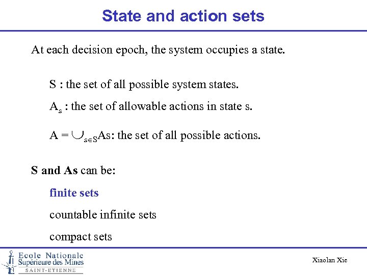State and action sets At each decision epoch, the system occupies a state. S : the set of all possible system states. As : the set of allowable actions in state s. A = s SAs: the set of all possible actions. S and As can be: finite sets countable infinite sets compact sets Xiaolan Xie

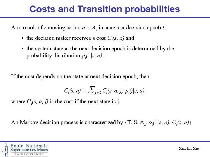Costs and Transition probabilities As a result of choosing action a As in state s at decision epoch t, • the decision maker receives a cost Ct(s, a) and • the system state at the next decision epoch is determined by the probability distribution pt(. |s, a). If the cost depends on the state at next decision epoch, then Ct(s, a) = j S Ct(s, a, j) pt(j|s, a). where Ct(s, a, j) is the cost if the next state is j. An Markov decision process is characterized by {T, S, As, pt(. |s, a), Ct(s, a)} Xiaolan Xie

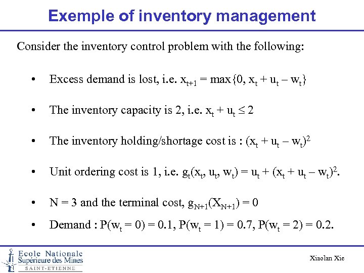Exemple of inventory management Consider the inventory control problem with the following: • Excess demand is lost, i. e. xt+1 = max{0, xt + ut – wt} • The inventory capacity is 2, i. e. xt + ut 2 • The inventory holding/shortage cost is : (xt + ut – wt)2 • Unit ordering cost is 1, i. e. gt(xt, ut, wt) = ut + (xt + ut – wt)2. • N = 3 and the terminal cost, g. N+1(XN+1) = 0 • Demand : P(wt = 0) = 0. 1, P(wt = 1) = 0. 7, P(wt = 2) = 0. 2. Xiaolan Xie

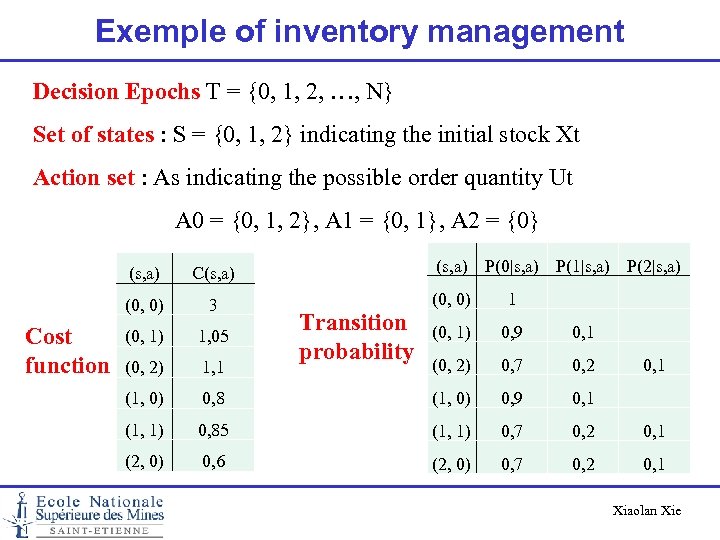Exemple of inventory management Decision Epochs T = {0, 1, 2, …, N} Set of states : S = {0, 1, 2} indicating the initial stock Xt Action set : As indicating the possible order quantity Ut A 0 = {0, 1, 2}, A 1 = {0, 1}, A 2 = {0} (s, a) (0, 0) Cost function 3 (0, 1) 1, 05 (0, 2) 1, 1 (1, 0) (s, a) P(0|s, a) P(1|s, a) P(2|s, a) C(s, a) (0, 0) 1 (0, 1) 0, 9 0, 1 (0, 2) 0, 7 0, 2 0, 8 (1, 0) 0, 9 0, 1 (1, 1) 0, 85 (1, 1) 0, 7 0, 2 0, 1 (2, 0) 0, 6 (2, 0) 0, 7 0, 2 0, 1 Transition probability 0, 1 Xiaolan Xie

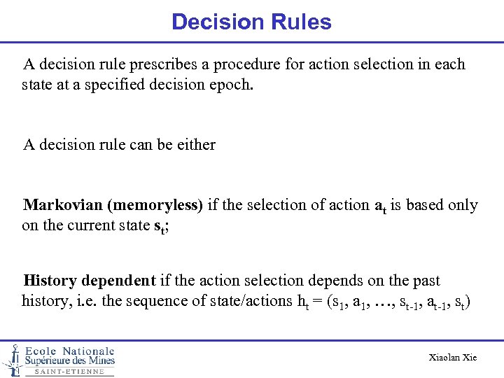Decision Rules A decision rule prescribes a procedure for action selection in each state at a specified decision epoch. A decision rule can be either Markovian (memoryless) if the selection of action at is based only on the current state st; History dependent if the action selection depends on the past history, i. e. the sequence of state/actions ht = (s 1, a 1, …, st-1, at-1, st) Xiaolan Xie

Decision Rules A decision rule can also be either Deterministic if the decision rule selects one action with certainty Randomized if the decision rule only specifies a probability distribution on the set of actions. Xiaolan Xie

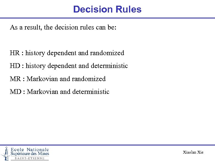Decision Rules As a result, the decision rules can be: HR : history dependent and randomized HD : history dependent and deterministic MR : Markovian and randomized MD : Markovian and deterministic Xiaolan Xie

Policies A policy specifies the decision rule to be used at all decision epoch. A policy p is a sequence of decision rules, i. e. p = {d 1, d 2, …, d. N-1} A policy is stationary if dt = d for all t. Stationary deterministic or stationary randomized policies are important for infinite horizon markov decision processes. Xiaolan Xie

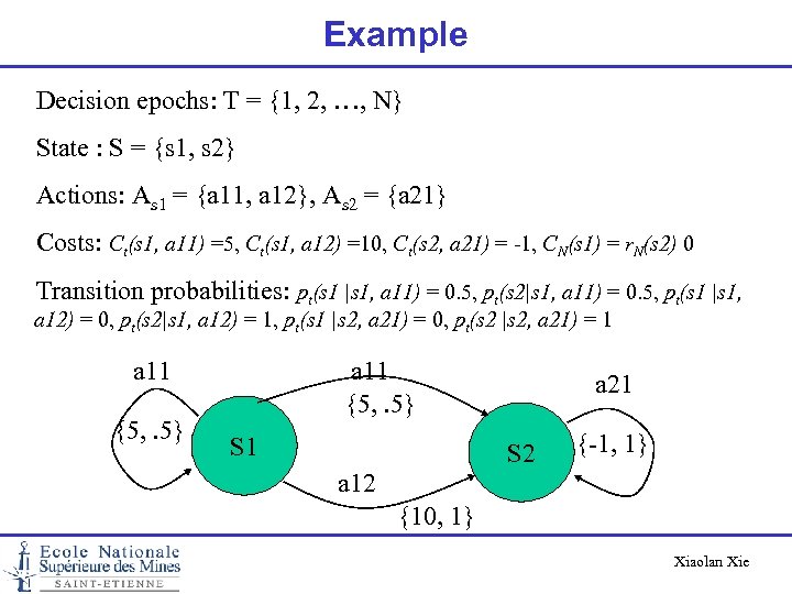Example Decision epochs: T = {1, 2, …, N} State : S = {s 1, s 2} Actions: As 1 = {a 11, a 12}, As 2 = {a 21} Costs: Ct(s 1, a 11) =5, Ct(s 1, a 12) =10, Ct(s 2, a 21) = -1, CN(s 1) = r. N(s 2) 0 Transition probabilities: pt(s 1 |s 1, a 11) = 0. 5, pt(s 2|s 1, a 11) = 0. 5, pt(s 1 |s 1, a 12) = 0, pt(s 2|s 1, a 12) = 1, pt(s 1 |s 2, a 21) = 0, pt(s 2 |s 2, a 21) = 1 a 11 {5, . 5} S 1 a 21 S 2 {-1, 1} a 12 {10, 1} Xiaolan Xie

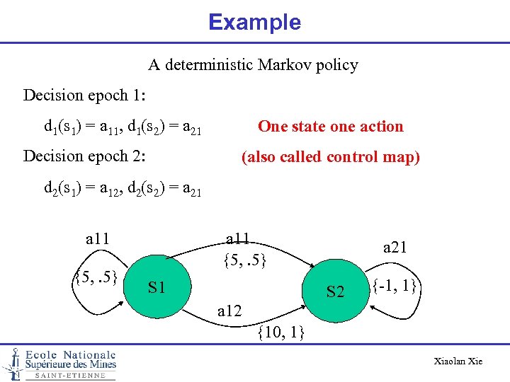Example A deterministic Markov policy Decision epoch 1: d 1(s 1) = a 11, d 1(s 2) = a 21 Decision epoch 2: One state one action (also called control map) d 2(s 1) = a 12, d 2(s 2) = a 21 a 11 {5, . 5} S 1 a 21 S 2 {-1, 1} a 12 {10, 1} Xiaolan Xie

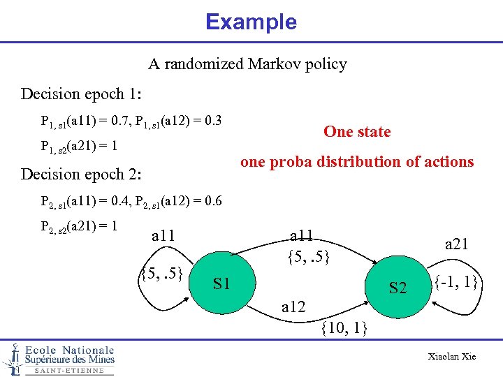Example A randomized Markov policy Decision epoch 1: P 1, s 1(a 11) = 0. 7, P 1, s 1(a 12) = 0. 3 P 1, s 2(a 21) = 1 One state one proba distribution of actions Decision epoch 2: P 2, s 1(a 11) = 0. 4, P 2, s 1(a 12) = 0. 6 P 2, s 2(a 21) = 1 a 11 {5, . 5} S 1 a 21 S 2 {-1, 1} a 12 {10, 1} Xiaolan Xie

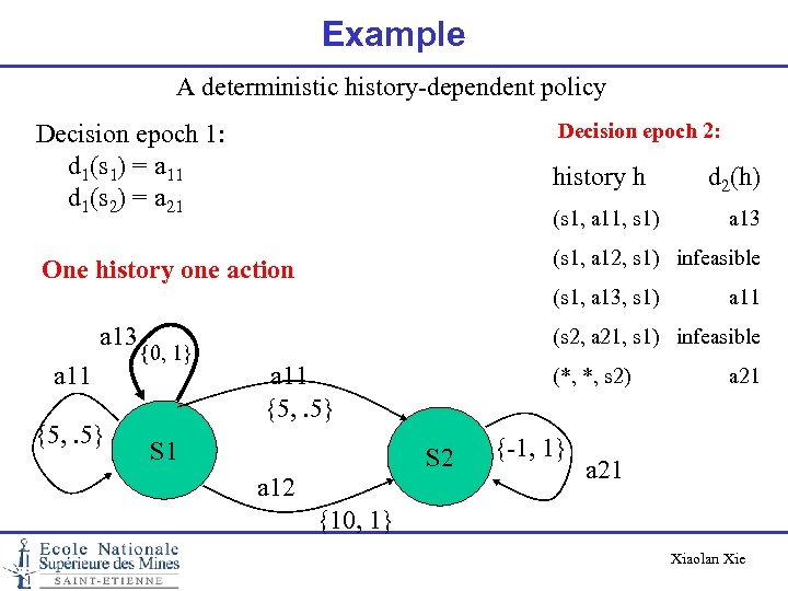Example A deterministic history-dependent policy Decision epoch 1: d 1(s 1) = a 11 d 1(s 2) = a 21 Decision epoch 2: One history one action (s 1, a 12, s 1) infeasible history h (s 1, a 11, s 1) (s 1, a 13, s 1) a 13 a 11 {5, . 5} {0, 1} d 2(h) a 13 a 11 (s 2, a 21, s 1) infeasible a 11 {5, . 5} S 1 (*, *, s 2) S 2 a 12 {-1, 1} a 21 {10, 1} Xiaolan Xie

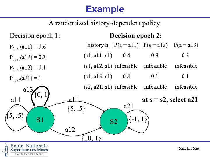Example A randomized history-dependent policy Decision epoch 1: Decision epoch 2: P 1, s 1(a 11) = 0. 6 history h P 1, s 1(a 12) = 0. 3 (s 1, a 11, s 1) P 1, s 1(a 12) = 0. 1 (s 1, a 12, s 1) infeasible P 1, s 2(a 21) = 1 (s 1, a 13, s 1) a 13 a 11 {5, . 5} P(a = a 11) P(a = a 12) P(a = a 13) 0. 4 0. 3 0. 8 0. 1 (s 2, a 21, s 1) infeasible {0, 1} a 11 {5, . 5} S 1 a 21 S 2 0. 3 infeasible 0. 1 infeasible at s = s 2, select a 21 {-1, 1} a 12 {10, 1} Xiaolan Xie

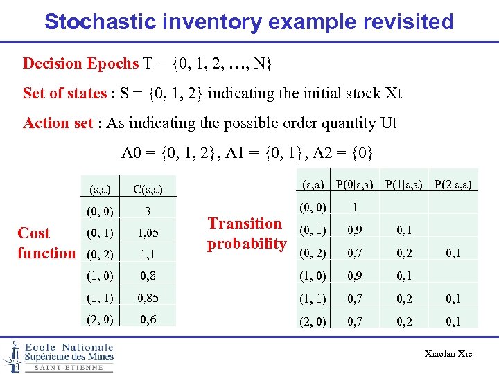Stochastic inventory example revisited Decision Epochs T = {0, 1, 2, …, N} Set of states : S = {0, 1, 2} indicating the initial stock Xt Action set : As indicating the possible order quantity Ut A 0 = {0, 1, 2}, A 1 = {0, 1}, A 2 = {0} (s, a) (0, 0) Cost function 3 (0, 1) 1, 05 (0, 2) 1, 1 (1, 0) (s, a) P(0|s, a) P(1|s, a) P(2|s, a) C(s, a) (0, 0) 1 (0, 1) 0, 9 0, 1 (0, 2) 0, 7 0, 2 0, 8 (1, 0) 0, 9 0, 1 (1, 1) 0, 85 (1, 1) 0, 7 0, 2 0, 1 (2, 0) 0, 6 (2, 0) 0, 7 0, 2 0, 1 Transition probability 0, 1 Xiaolan Xie

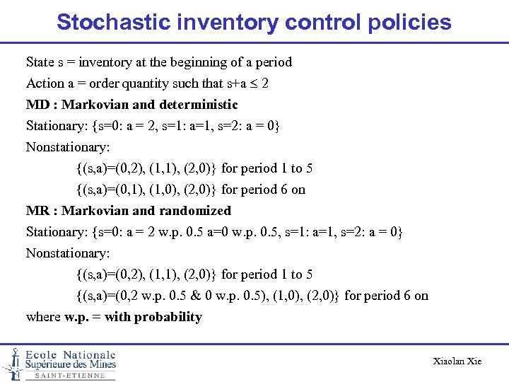Stochastic inventory control policies State s = inventory at the beginning of a period Action a = order quantity such that s+a 2 MD : Markovian and deterministic Stationary: {s=0: a = 2, s=1: a=1, s=2: a = 0} Nonstationary: {(s, a)=(0, 2), (1, 1), (2, 0)} for period 1 to 5 {(s, a)=(0, 1), (1, 0), (2, 0)} for period 6 on MR : Markovian and randomized Stationary: {s=0: a = 2 w. p. 0. 5 a=0 w. p. 0. 5, s=1: a=1, s=2: a = 0} Nonstationary: {(s, a)=(0, 2), (1, 1), (2, 0)} for period 1 to 5 {(s, a)=(0, 2 w. p. 0. 5 & 0 w. p. 0. 5), (1, 0), (2, 0)} for period 6 on where w. p. = with probability Xiaolan Xie

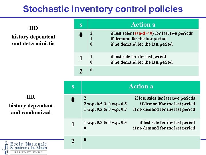Stochastic inventory control policies s 0 HD history dependent and deterministic Action a 2 1 0 if lost sales (s+a-d < 0) for last two periods if demand for the last period if no demand for the last period 1 1 0 if lost sale for the last period if no demand for the last period 2 0 s HR history dependent and randomized Action a 0 2 if lost sales for last two periods 2 w. p. 0. 5 & 0 w. p. 0. 5 if demandfor the last period 1 w. p. 0. 3 & 0 w. p. 0. 7 if no demand for the last period 1 1 w. p. 0. 5 & 0 w. p. 0. 5 0 2 0 if lost sale for the last period if no demand for the last period Xiaolan Xie

Remarks Each Markov policy leads to a discrete time Markov Chain and the policy can be evaluated by solving the related Markov chain. Xiaolan Xie

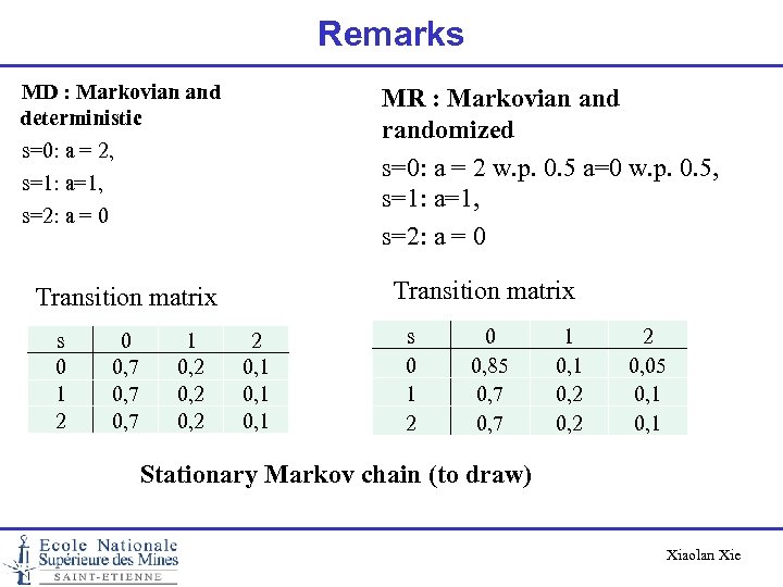Remarks MD : Markovian and deterministic s=0: a = 2, s=1: a=1, s=2: a = 0 MR : Markovian and randomized s=0: a = 2 w. p. 0. 5 a=0 w. p. 0. 5, s=1: a=1, s=2: a = 0 Transition matrix s 0 1 2 0 0, 7 1 0, 2 2 0, 1 s 0 1 2 0 0, 85 0, 7 1 0, 2 2 0, 05 0, 1 Stationary Markov chain (to draw) Xiaolan Xie

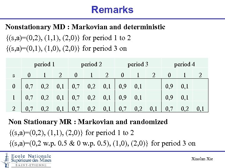Remarks Nonstationary MD : Markovian and deterministic {(s, a)=(0, 2), (1, 1), (2, 0)} for period 1 to 2 {(s, a)=(0, 1), (1, 0), (2, 0)} for period 3 on period 1 period 2 period 3 period 4 s 0 1 2 0 0, 7 0, 2 0, 1 0, 9 0, 1 1 0, 7 0, 2 0, 1 0, 9 0, 1 2 0, 7 0, 2 0, 1 Non Stationary MR : Markovian and randomized {(s, a)=(0, 2), (1, 1), (2, 0)} for period 1 to 2 {(s, a)=(0, 2 w. p. 0. 5 & 0 w. p. 0. 5), (1, 0), (2, 0)} for period 3 on Xiaolan Xie

Finite Horizon Markov Decision Processes Xiaolan Xie

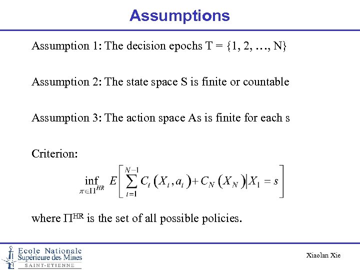Assumptions Assumption 1: The decision epochs T = {1, 2, …, N} Assumption 2: The state space S is finite or countable Assumption 3: The action space As is finite for each s Criterion: where PHR is the set of all possible policies. Xiaolan Xie

Optimality of Markov deterministic policy Theorem : Assume S is finite or countable, and that As is finite for each s S. Then there exists a Markovian deterministic policy which is optimal. Xiaolan Xie

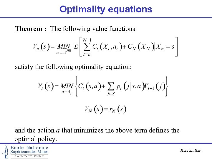Optimality equations Theorem : The following value functions satisfy the following optimality equation: and the action a that minimizes the above term defines the optimal policy. Xiaolan Xie

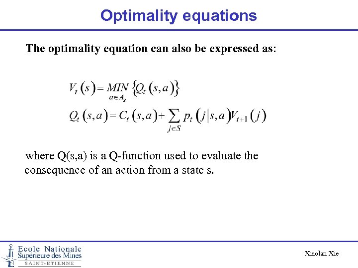Optimality equations The optimality equation can also be expressed as: where Q(s, a) is a Q-function used to evaluate the consequence of an action from a state s. Xiaolan Xie

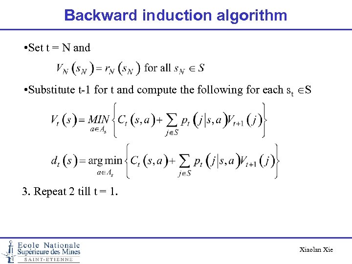Backward induction algorithm • Set t = N and • Substitute t-1 for t and compute the following for each st S 3. Repeat 2 till t = 1. Xiaolan Xie

Infinite Horizon discounted Markov decision processes Xiaolan Xie

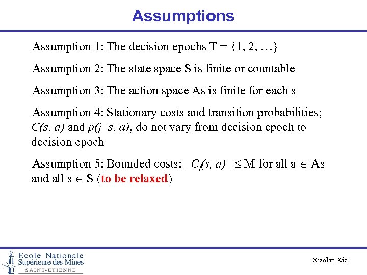Assumptions Assumption 1: The decision epochs T = {1, 2, …} Assumption 2: The state space S is finite or countable Assumption 3: The action space As is finite for each s Assumption 4: Stationary costs and transition probabilities; C(s, a) and p(j |s, a), do not vary from decision epoch to decision epoch Assumption 5: Bounded costs: | Ct(s, a) | M for all a As and all s S (to be relaxed) Xiaolan Xie

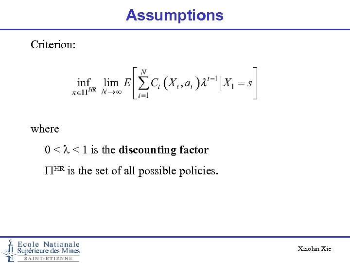Assumptions Criterion: where 0 < l < 1 is the discounting factor PHR is the set of all possible policies. Xiaolan Xie

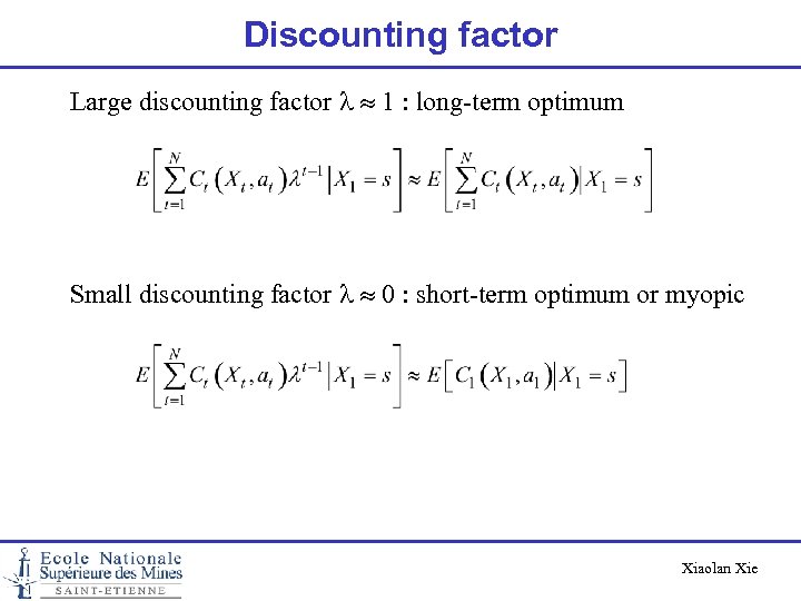Discounting factor Large discounting factor l 1 : long-term optimum Small discounting factor l 0 : short-term optimum or myopic Xiaolan Xie

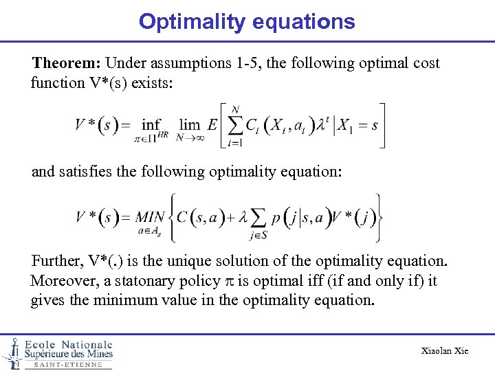Optimality equations Theorem: Under assumptions 1 -5, the following optimal cost function V*(s) exists: and satisfies the following optimality equation: Further, V*(. ) is the unique solution of the optimality equation. Moreover, a statonary policy p is optimal iff (if and only if) it gives the minimum value in the optimality equation. Xiaolan Xie

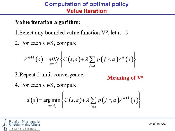Computation of optimal policy Value Iteration Value iteration algorithm: 1. Select any bounded value function V 0, let n =0 2. For each s S, compute 3. Repeat 2 until convergence. Meaning of Vn 4. For each s S, compute Xiaolan Xie

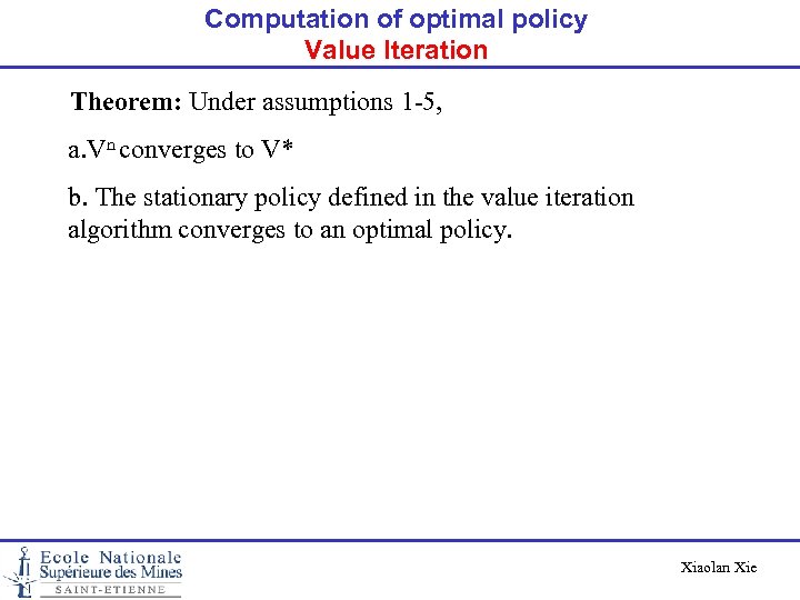Computation of optimal policy Value Iteration Theorem: Under assumptions 1 -5, a. Vn converges to V* b. The stationary policy defined in the value iteration algorithm converges to an optimal policy. Xiaolan Xie

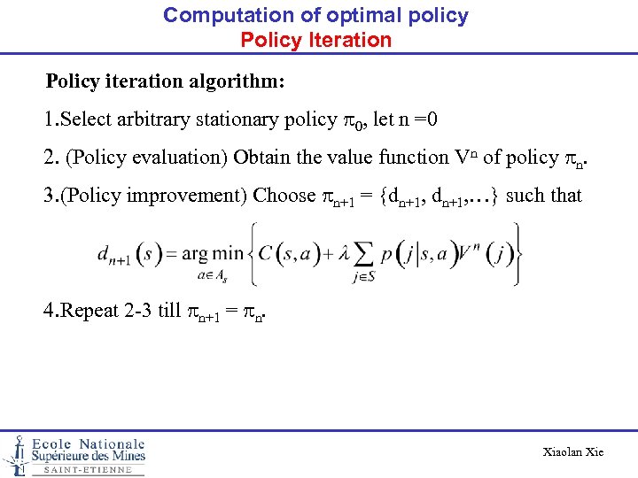Computation of optimal policy Policy Iteration Policy iteration algorithm: 1. Select arbitrary stationary policy p 0, let n =0 2. (Policy evaluation) Obtain the value function Vn of policy pn. 3. (Policy improvement) Choose pn+1 = {dn+1, …} such that 4. Repeat 2 -3 till pn+1 = pn. Xiaolan Xie

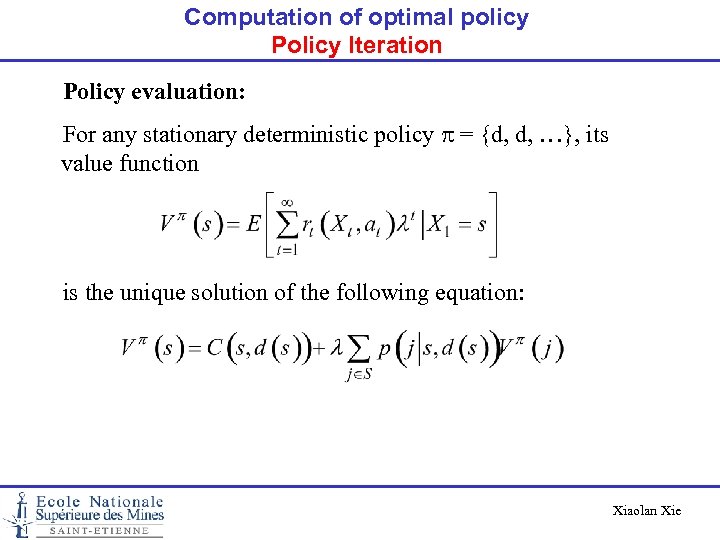Computation of optimal policy Policy Iteration Policy evaluation: For any stationary deterministic policy p = {d, d, …}, its value function is the unique solution of the following equation: Xiaolan Xie

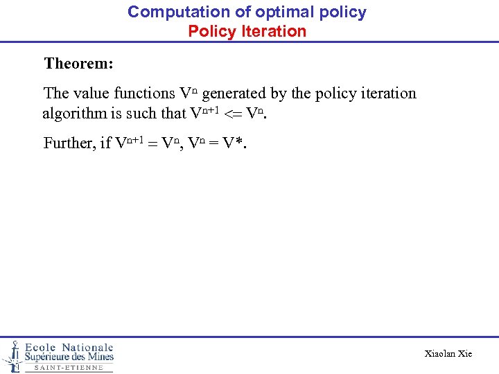Computation of optimal policy Policy Iteration Theorem: The value functions Vn generated by the policy iteration algorithm is such that Vn+1 <= Vn. Further, if Vn+1 = Vn, Vn = V*. Xiaolan Xie

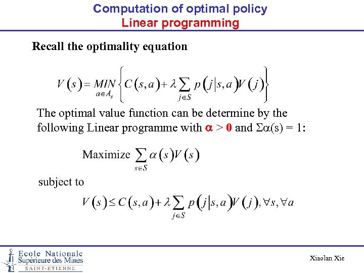Computation of optimal policy Linear programming Recall the optimality equation The optimal value function can be determine by the following Linear programme with a > 0 and Sa(s) = 1: Xiaolan Xie

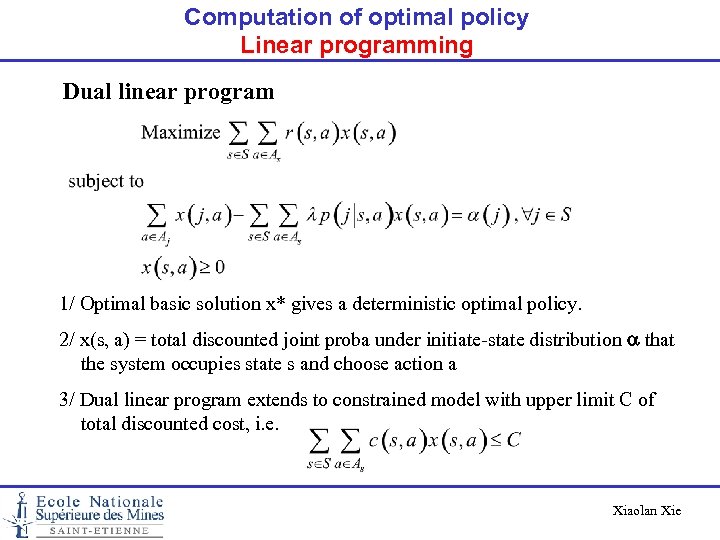Computation of optimal policy Linear programming Dual linear program 1/ Optimal basic solution x* gives a deterministic optimal policy. 2/ x(s, a) = total discounted joint proba under initiate-state distribution a that the system occupies state s and choose action a 3/ Dual linear program extends to constrained model with upper limit C of total discounted cost, i. e. Xiaolan Xie

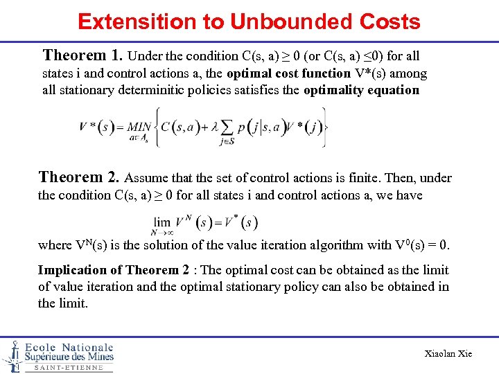Extensition to Unbounded Costs Theorem 1. Under the condition C(s, a) ≥ 0 (or C(s, a) ≤ 0) for all states i and control actions a, the optimal cost function V*(s) among all stationary determinitic policies satisfies the optimality equation Theorem 2. Assume that the set of control actions is finite. Then, under the condition C(s, a) ≥ 0 for all states i and control actions a, we have where VN(s) is the solution of the value iteration algorithm with V 0(s) = 0. Implication of Theorem 2 : The optimal cost can be obtained as the limit of value iteration and the optimal stationary policy can also be obtained in the limit. Xiaolan Xie

Example • Consider a computer system consisting of M different processors. • Using processor i for a job incurs a finite cost Ci with C 1 < C 2 <. . . < CM. • When we submit a job to this system, processor i is assigned to our job with probability pi. • At this point we can (a) decide to go with this processor or (b) choose to hold the job until a lower-cost processor is assigned. • The system periodically return to our job and assign a processor in the same way. • Waiting until the next processor assignment incurs a fixed finite cost c. Question: How do we decide to go with the processor currently assigned to our job versus waiting for the next assignment? Suggestions: • The state definition should include all information useful for decision • The problem belongs to the so-called stochastic shortest path problem. Xiaolan Xie

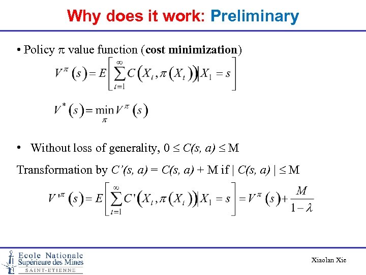Why does it work: Preliminary • Policy p value function (cost minimization) • Without loss of generality, 0 C(s, a) M Transformation by C’(s, a) = C(s, a) + M if | C(s, a) | M Xiaolan Xie

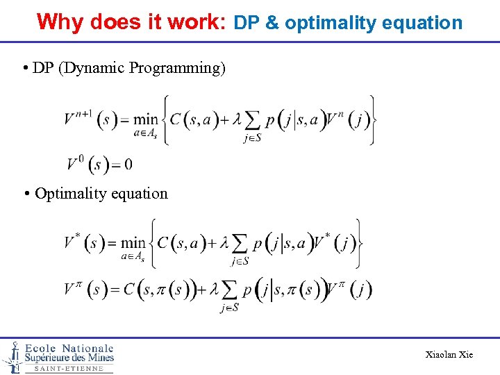Why does it work: DP & optimality equation • DP (Dynamic Programming) • Optimality equation Xiaolan Xie

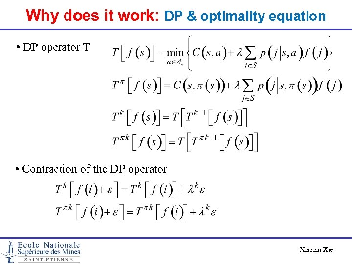Why does it work: DP & optimality equation • DP operator T • Contraction of the DP operator Xiaolan Xie

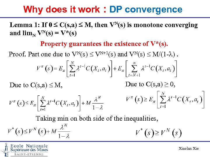Why does it work : DP convergence Lemma 1: If 0 C(s, a) M, then VN(s) is monotone converging and lim. N VN(s) = V*(s) Property guarantees the existence of V*(s). Proof. Part one due to VN(s) VN+1(s) and VN(s) M/(1 -l). Due to C(s, a) M, Due to C(s, a) ≥ 0, Taking min on both side of the inequalities, Xiaolan Xie

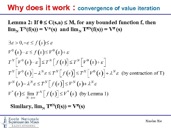Why does it work : convergence of value iteration Lemma 2: If 0 C(s, a) M, for any bounded function f, then lim. N TN(f(s)) = V*(s) and lim. N Tp. N(f(s)) = Vp (s) Similary, lim. N Tp. N(f(s)) = Vp(s) Xiaolan Xie

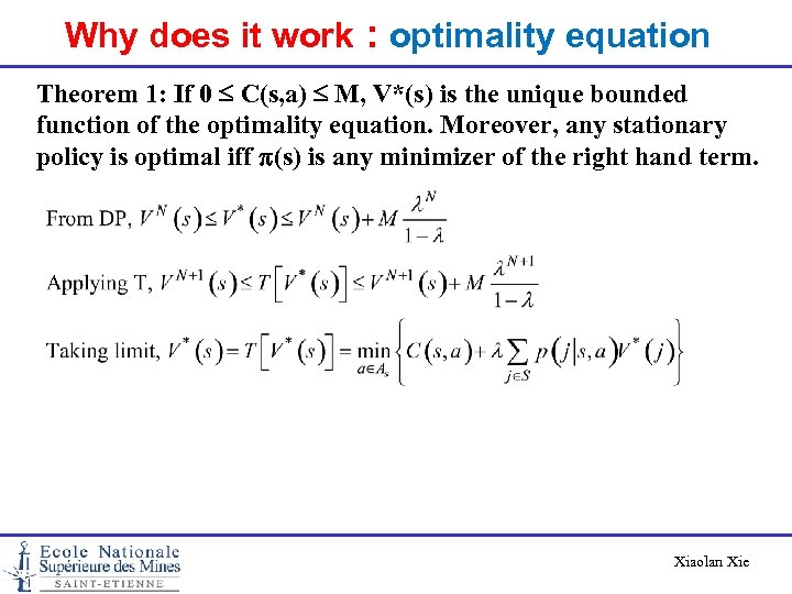Why does it work : optimality equation Theorem 1: If 0 C(s, a) M, V*(s) is the unique bounded function of the optimality equation. Moreover, any stationary policy is optimal iff p(s) is any minimizer of the right hand term. Xiaolan Xie

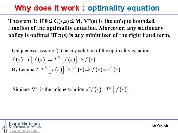Why does it work : optimality equation Theorem 1: If 0 C(s, a) M, V*(s) is the unique bounded function of the optimality equation. Moreover, any stationary policy is optimal iff p(s) is any minimizer of the right hand term. Xiaolan Xie

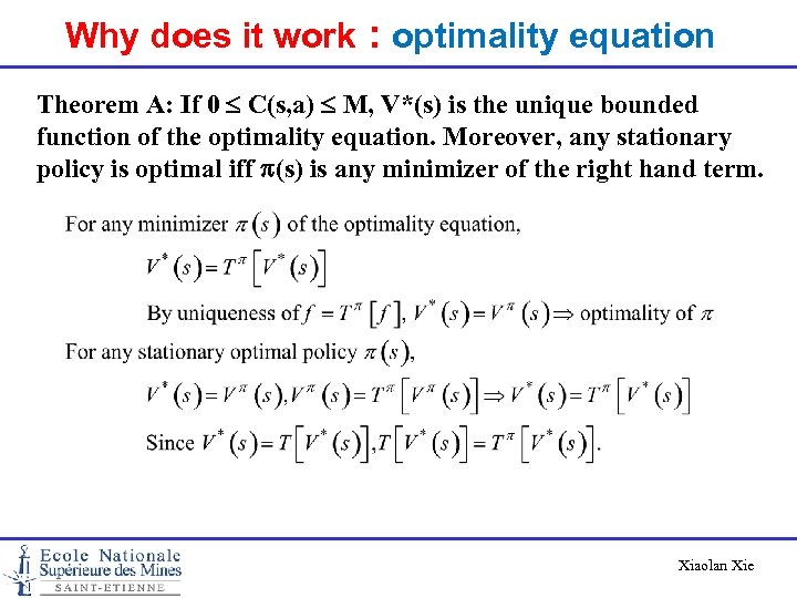Why does it work : optimality equation Theorem A: If 0 C(s, a) M, V*(s) is the unique bounded function of the optimality equation. Moreover, any stationary policy is optimal iff p(s) is any minimizer of the right hand term. Xiaolan Xie

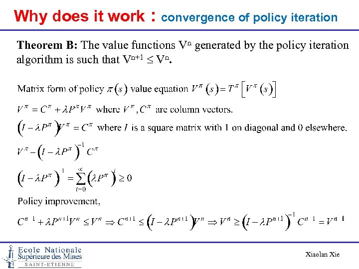Why does it work : convergence of policy iteration Theorem B: The value functions Vn generated by the policy iteration algorithm is such that Vn+1 Vn. Xiaolan Xie

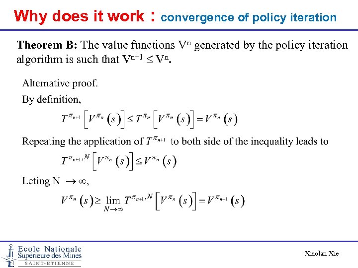Why does it work : convergence of policy iteration Theorem B: The value functions Vn generated by the policy iteration algorithm is such that Vn+1 Vn. Xiaolan Xie

Infinite Horizon average cost Markov decision processes Xiaolan Xie

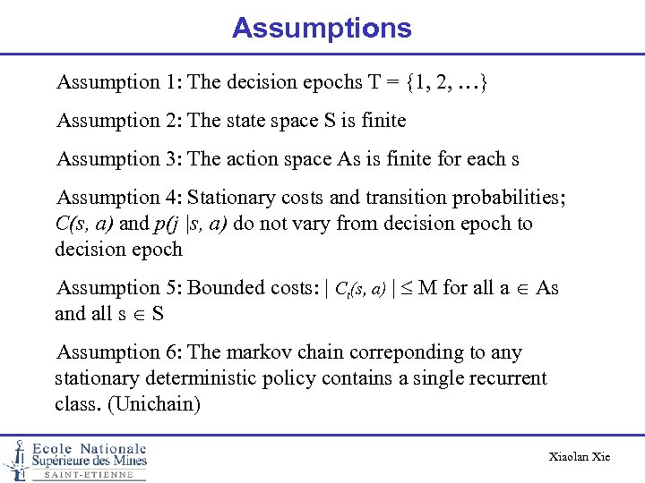Assumptions Assumption 1: The decision epochs T = {1, 2, …} Assumption 2: The state space S is finite Assumption 3: The action space As is finite for each s Assumption 4: Stationary costs and transition probabilities; C(s, a) and p(j |s, a) do not vary from decision epoch to decision epoch Assumption 5: Bounded costs: | Ct(s, a) | M for all a As and all s S Assumption 6: The markov chain correponding to any stationary deterministic policy contains a single recurrent class. (Unichain) Xiaolan Xie

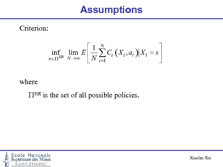Assumptions Criterion: where PHR is the set of all possible policies. Xiaolan Xie

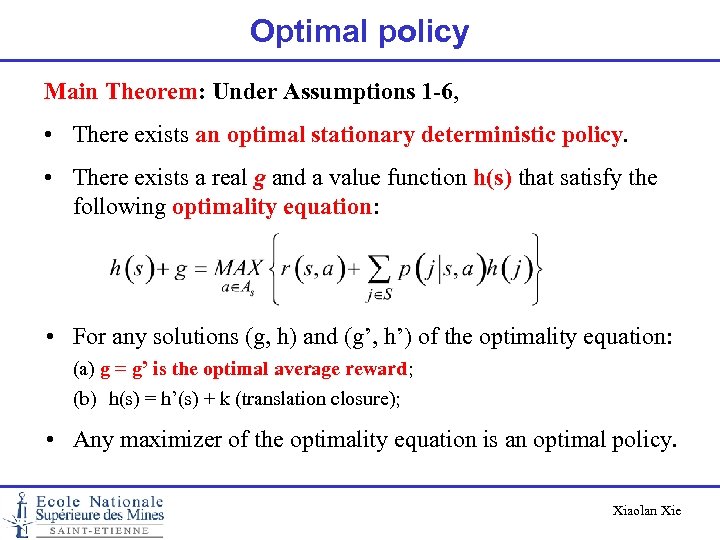Optimal policy Main Theorem: Under Assumptions 1 -6, • There exists an optimal stationary deterministic policy. • There exists a real g and a value function h(s) that satisfy the following optimality equation: • For any solutions (g, h) and (g’, h’) of the optimality equation: (a) g = g’ is the optimal average reward; (b) h(s) = h’(s) + k (translation closure); • Any maximizer of the optimality equation is an optimal policy. Xiaolan Xie

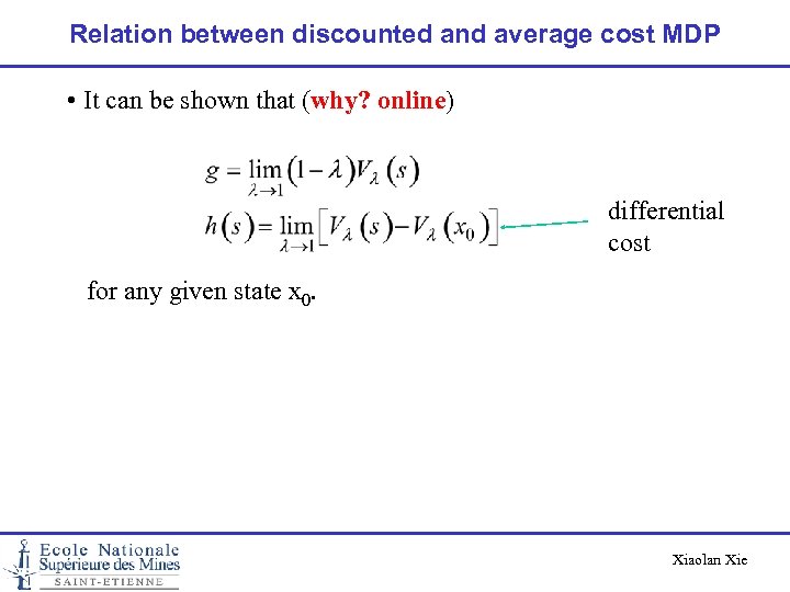Relation between discounted and average cost MDP • It can be shown that (why? online) differential cost for any given state x 0. Xiaolan Xie

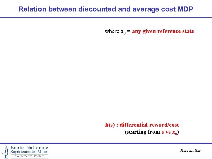Relation between discounted and average cost MDP where x 0 = any given reference state h(s) : differential reward/cost (starting from s vs x 0) Xiaolan Xie

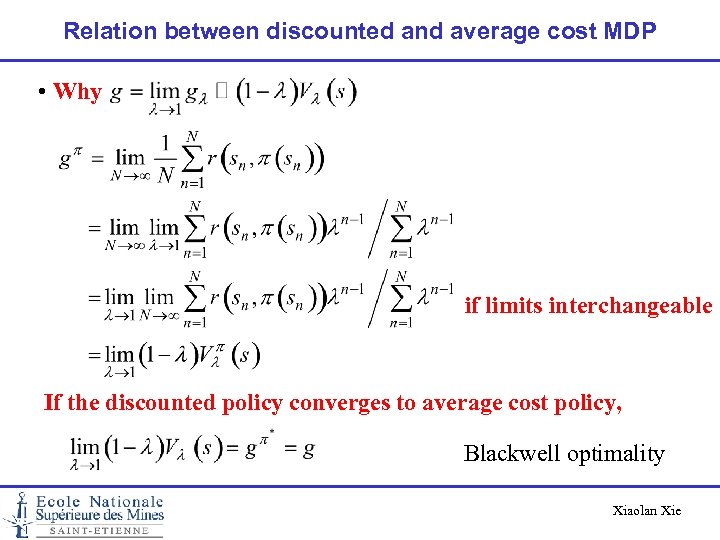Relation between discounted and average cost MDP • Why if limits interchangeable If the discounted policy converges to average cost policy, Blackwell optimality Xiaolan Xie

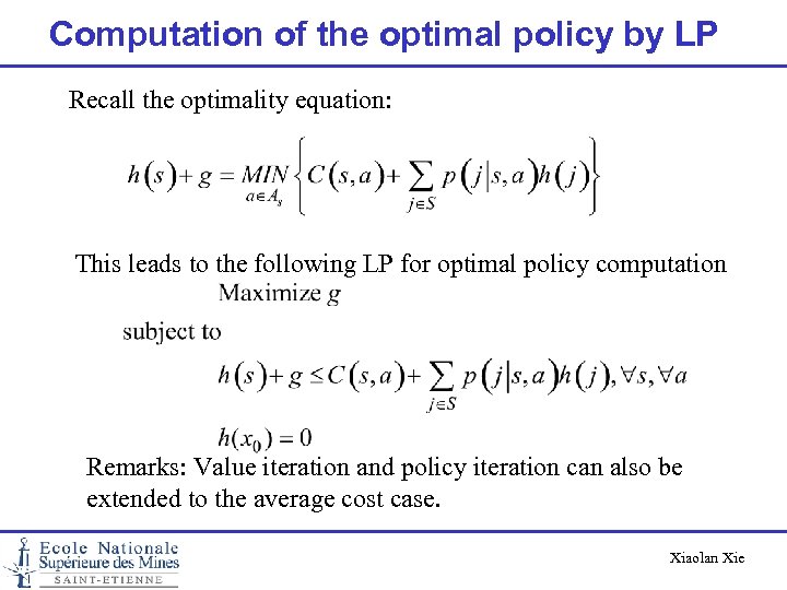Computation of the optimal policy by LP Recall the optimality equation: This leads to the following LP for optimal policy computation Remarks: Value iteration and policy iteration can also be extended to the average cost case. Xiaolan Xie

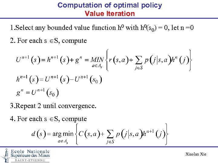Computation of optimal policy Value Iteration 1. Select any bounded value function h 0 with h 0(s 0) = 0, let n =0 2. For each s S, compute 3. Repeat 2 until convergence. 4. For each s S, compute Xiaolan Xie

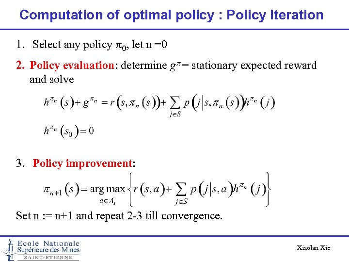Computation of optimal policy : Policy Iteration 1. Select any policy p 0, let n =0 2. Policy evaluation: determine gp = stationary expected reward and solve 3. Policy improvement: Set n : = n+1 and repeat 2 -3 till convergence. Xiaolan Xie

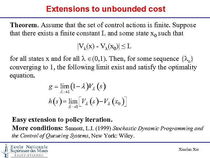Extensions to unbounded cost Theorem. Assume that the set of control actions is finite. Suppose that there exists a finite constant L and some state x 0 such that |Vl(x) - Vl(x 0)| ≤ L for all states x and for all l (0, 1). Then, for some sequence {ln} converging to 1, the following limit exist and satisfy the optimality equation. Easy extension to policy iteration. More conditions: Sennott, L. I. (1999) Stochastic Dynamic Programming and the Control of Queueing Systems, New York: Wiley. Xiaolan Xie

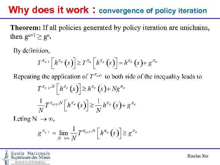Why does it work : convergence of policy iteration Theorem: If all policies generated by policy iteration are unichains, then gn+1 ≥ gn. Xiaolan Xie

Continuous time Markov decision processes Xiaolan Xie

Assumptions Assumption 1: The decision epochs T = R+ Assumption 2: The state space S is finite Assumption 3: The action space As is finite for each s Assumption 4: Stationary cost rates and transition rates; C(s, a) and m(j |s, a) do not vary from decision epoch to decision epoch Xiaolan Xie

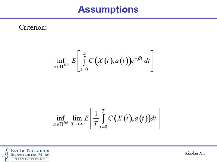Assumptions Criterion: Xiaolan Xie

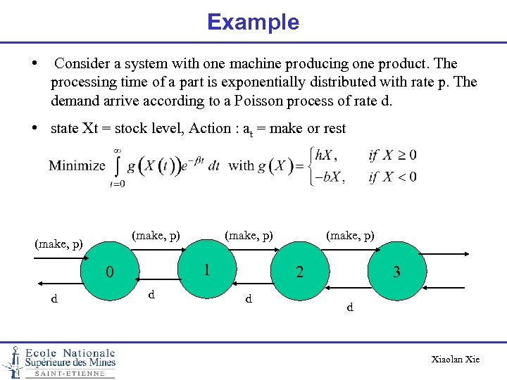Example • Consider a system with one machine producing one product. The processing time of a part is exponentially distributed with rate p. The demand arrive according to a Poisson process of rate d. • state Xt = stock level, Action : at = make or rest (make, p) 1 0 d (make, p) 2 d 3 d Xiaolan Xie

Uniformization Any continuous-time Markov chain can be converted to a discrete-time chain through a process called « uniformization » . Each Continuous Time Markov Chain is characterized by the transition rates mij of all possible transitions. The sojourn time Ti in each state i is exponentially distributed with rate m(i) = Sj≠i mij, i. e. E[Ti] = 1/m(i) Transitions different states are unpaced and asynchronuous depending on m(i). Xiaolan Xie

Uniformization In order to synchronize (uniformize) the transitions at the same pace, we choose a uniformization rate g MAX{m(i)} « Uniformized » Markov chain with • transitions occur only at instants generated by a common a Poisson process of rate g (also called standard clock) • state-transition probabilities pij = mij / g pii = 1 - m(i)/ g where the self-loop transitions correspond to fictitious events. Xiaolan Xie

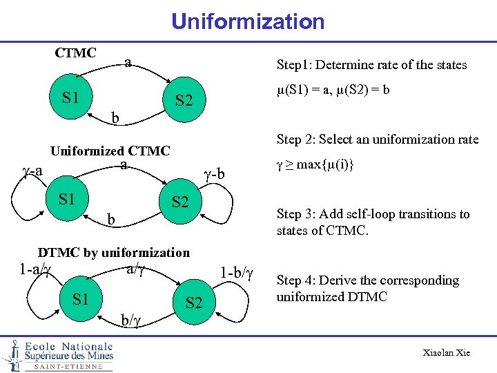Uniformization CTMC a S 1 Step 1: Determine rate of the states m(S 1) = a, m(S 2) = b S 2 b Step 2: Select an uniformization rate Uniformized CTMC a g-a S 1 g-b S 2 b g ≥ max{m(i)} Step 3: Add self-loop transitions to states of CTMC. DTMC by uniformization a/g 1 -a/g S 1 b/g 1 -b/g S 2 Step 4: Derive the corresponding uniformized DTMC Xiaolan Xie

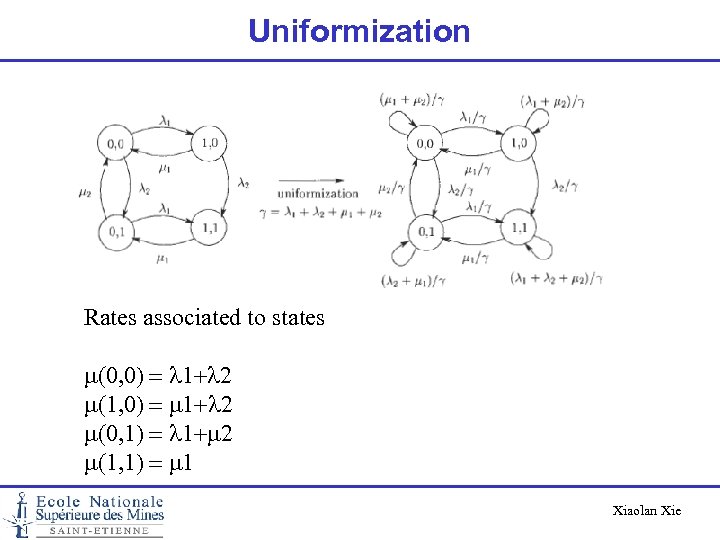Uniformization Rates associated to states m(0, 0) = l 1+l 2 m(1, 0) = m 1+l 2 m(0, 1) = l 1+m 2 m(1, 1) = m 1 Xiaolan Xie

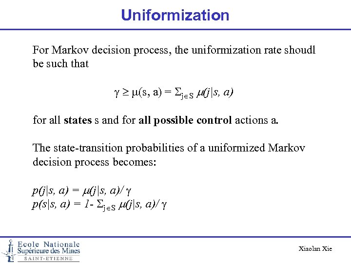Uniformization For Markov decision process, the uniformization rate shoudl be such that g m(s, a) = Sj S m(j|s, a) for all states s and for all possible control actions a. The state-transition probabilities of a uniformized Markov decision process becomes: p(j|s, a) = m(j|s, a)/ g p(s|s, a) = 1 - Sj S m(j|s, a)/ g Xiaolan Xie

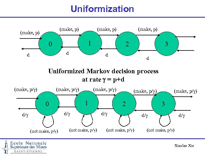Uniformization (make, p) 1 0 2 d d (make, p) 3 d d Uniformized Markov decision process at rate g = p+d (make, p/g) 1 0 d/g (not make, p/g) (make, p/g) 2 d/g (not make, p/g) (make, p/g) 3 d/g (not make, p/g) Xiaolan Xie

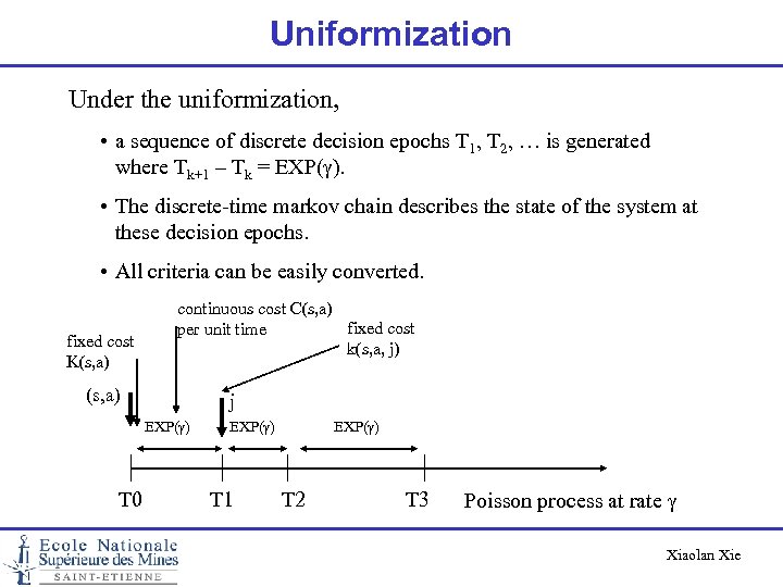Uniformization Under the uniformization, • a sequence of discrete decision epochs T 1, T 2, … is generated where Tk+1 – Tk = EXP(g). • The discrete-time markov chain describes the state of the system at these decision epochs. • All criteria can be easily converted. fixed cost K(s, a) continuous cost C(s, a) fixed cost per unit time k(s, a, j) (s, a) j EXP(g) T 0 EXP(g) T 1 EXP(g) T 2 T 3 Poisson process at rate g Xiaolan Xie

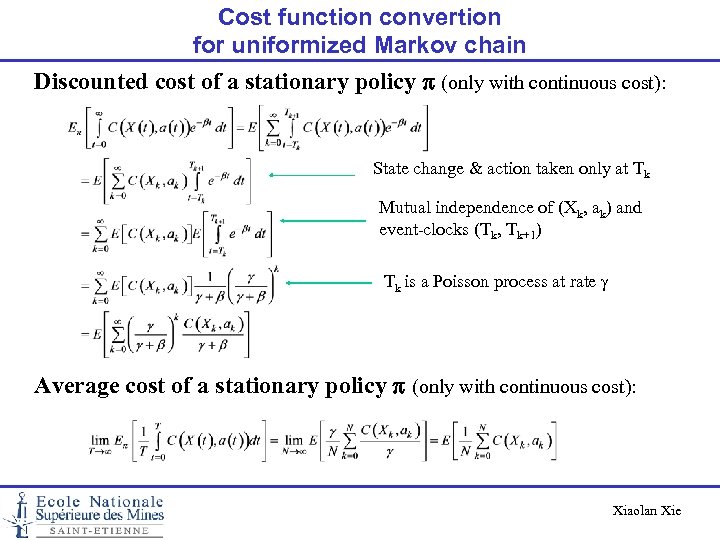Cost function convertion for uniformized Markov chain Discounted cost of a stationary policy p (only with continuous cost): State change & action taken only at Tk Mutual independence of (Xk, ak) and event-clocks (Tk, Tk+1) Tk is a Poisson process at rate g Average cost of a stationary policy p (only with continuous cost): Xiaolan Xie

Cost function convertion for uniformized Markov chain Tk is a Poisson process at rate g, i. e. Tk = t 1 + … + tk, ti = EXP(g) Xiaolan Xie

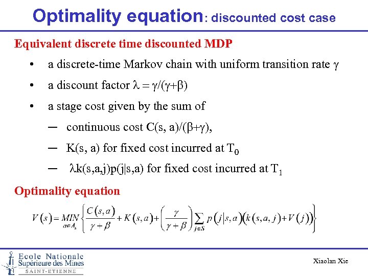Optimality equation: discounted cost case Equivalent discrete time discounted MDP • a discrete-time Markov chain with uniform transition rate g • a discount factor l = g/(g+b) • a stage cost given by the sum of ─ continuous cost C(s, a)/(b+g), ─ K(s, a) for fixed cost incurred at T 0 ─ lk(s, a, j)p(j|s, a) for fixed cost incurred at T 1 Optimality equation Xiaolan Xie

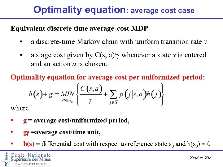Optimality equation: average cost case Equivalent discrete time average-cost MDP • a discrete-time Markov chain with uniform transition rate g • a stage cost given by C(s, a)/g whenever a state s is entered an action a is chosen. Optimality equation for average cost per uniformized period: where • g = average cost/uniformized period, • gg =average cost/time unit, • h(s) = differential cost with respect to reference state s 0 and h(s 0) = 0 Xiaolan Xie

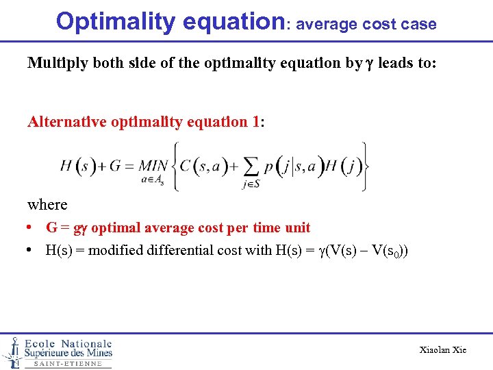Optimality equation: average cost case Multiply both side of the optimality equation by g leads to: Alternative optimality equation 1: where • G = gg optimal average cost per time unit • H(s) = modified differential cost with H(s) = g(V(s) – V(s 0)) Xiaolan Xie

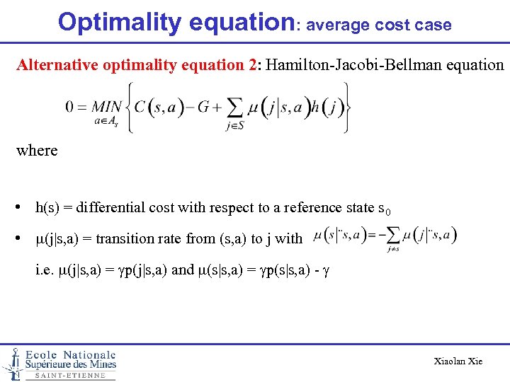Optimality equation: average cost case Alternative optimality equation 2: Hamilton-Jacobi-Bellman equation where • h(s) = differential cost with respect to a reference state s 0 • m(j|s, a) = transition rate from (s, a) to j with i. e. m(j|s, a) = gp(j|s, a) and m(s|s, a) = gp(s|s, a) - g Xiaolan Xie

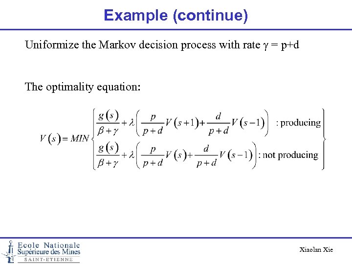Example (continue) Uniformize the Markov decision process with rate g = p+d The optimality equation: Xiaolan Xie

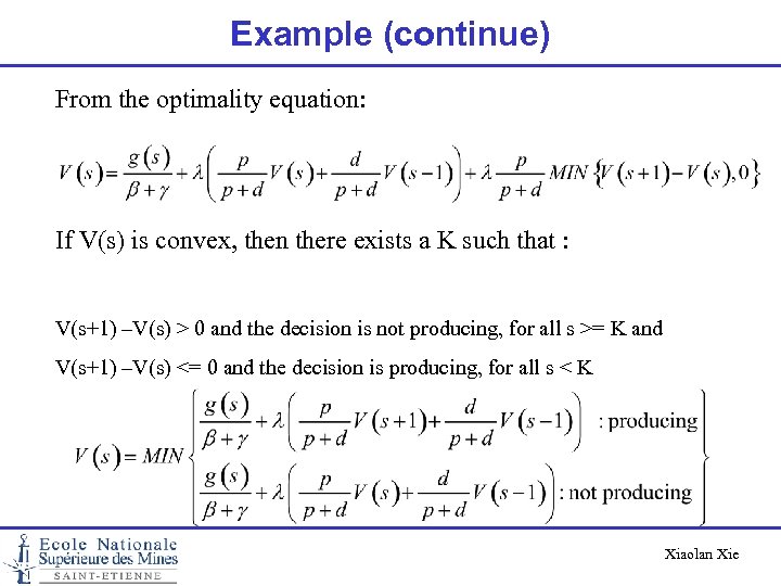Example (continue) From the optimality equation: If V(s) is convex, then there exists a K such that : V(s+1) –V(s) > 0 and the decision is not producing, for all s >= K and V(s+1) –V(s) <= 0 and the decision is producing, for all s < K Xiaolan Xie

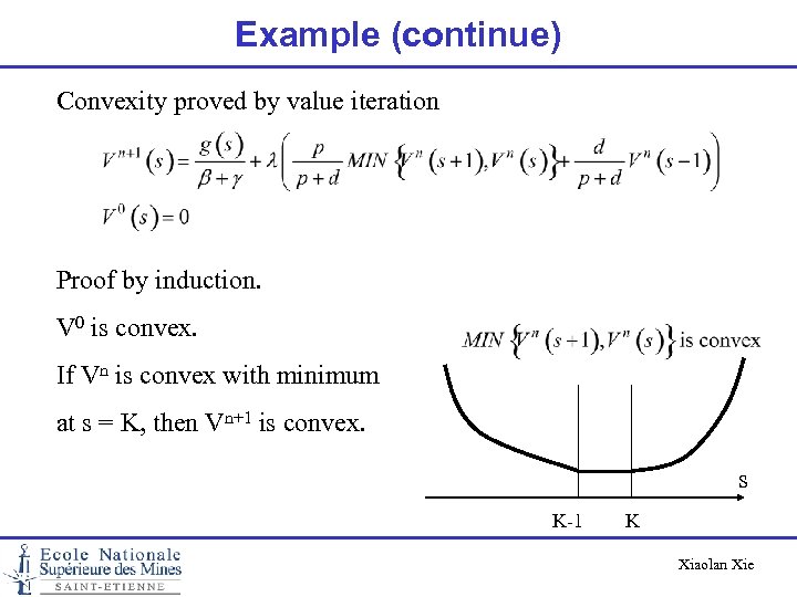Example (continue) Convexity proved by value iteration Proof by induction. V 0 is convex. If Vn is convex with minimum at s = K, then Vn+1 is convex. s K-1 K Xiaolan Xie

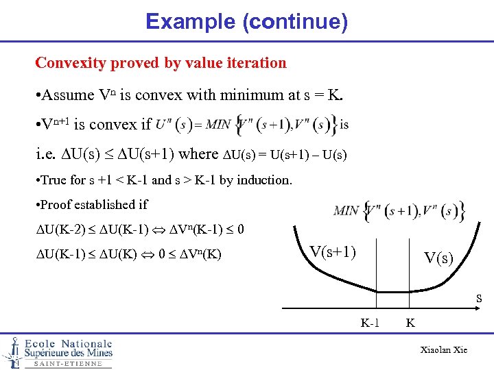Example (continue) Convexity proved by value iteration • Assume Vn is convex with minimum at s = K. • Vn+1 is convex if i. e. DU(s) DU(s+1) where DU(s) = U(s+1) – U(s) • True for s +1 < K-1 and s > K-1 by induction. • Proof established if DU(K-2) DU(K-1) DVn(K-1) 0 DU(K-1) DU(K) 0 DVn(K) V(s+1) V(s) s K-1 K Xiaolan Xie

Condition for optimality of monotone policy (first order properties) Xiaolan Xie

Monotone policy p(s) nondecreasing or nonincreasing in s Question: When there exists an optimal monotone policy? Answers: monotonicity (addressed here) and convexity (addressed in the previous example) Only finite-horizon case is considered but can be extented to discounted and average cost. Xiaolan Xie

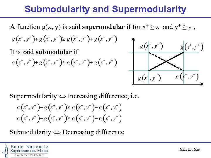Submodularity and Supermodularity A function g(x, y) is said supermodular if for x+ ≥ x- and y+ ≥ y-, It is said submodular if Supermodularity Increasing difference, i. e. Submodularity Decreasing difference Xiaolan Xie

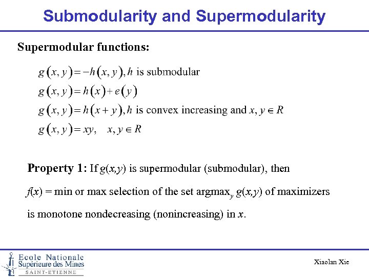Submodularity and Supermodularity Supermodular functions: Property 1: If g(x, y) is supermodular (submodular), then f(x) = min or max selection of the set argmaxy g(x, y) of maximizers is monotone nondecreasing (nonincreasing) in x. Xiaolan Xie

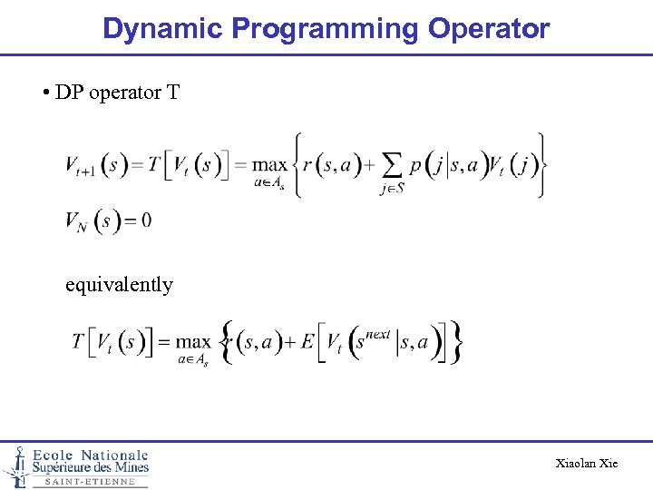Dynamic Programming Operator • DP operator T equivalently Xiaolan Xie

DP Operator: monotonicity preservation Property 2 T[Vt(s)] is nondecreasing (nonincreasing) if 1. r(s, a) is nondecreasing (nonincreasing) in s for all a 2. (snext|s, a) is nondecreasing in s for all a, k Xiaolan Xie

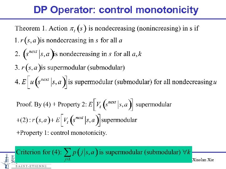DP Operator: control monotonicity Xiaolan Xie

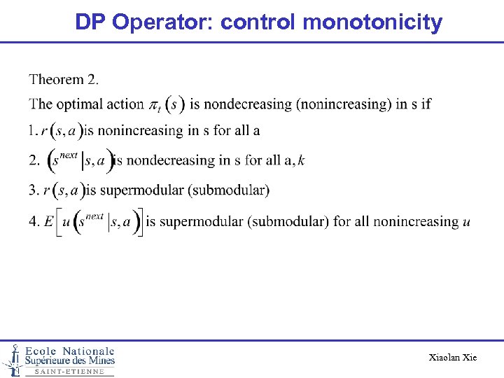DP Operator: control monotonicity Xiaolan Xie

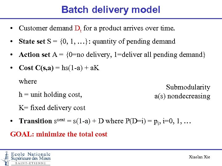Batch delivery model • Customer demand Dt for a product arrives over time. • State set S = {0, 1, …}: quantity of pending demand • Action set A = {0=no delivery, 1=deliver all pending demand} • Cost C(s, a) = hs(1 -a) + a. K where h = unit holding cost, Submodularity a(s) nondecreasing K= fixed delivery cost • Transition snext = s(1 -a) + D where P(D=i) = pi, i=0, 1, … GOAL: minimize the total cost Xiaolan Xie

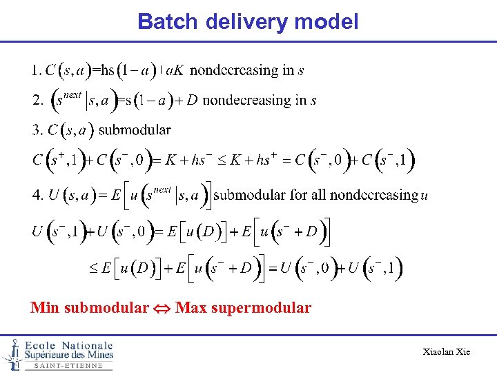Batch delivery model Min submodular Max supermodular Xiaolan Xie

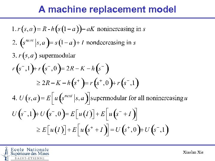
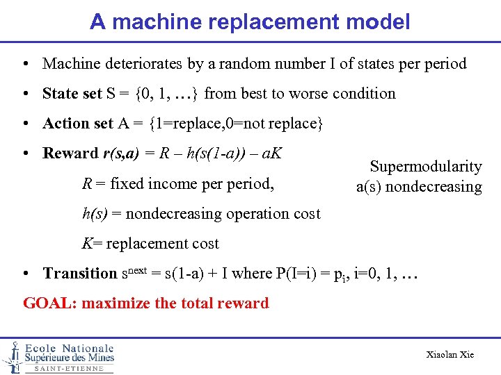A machine replacement model • Machine deteriorates by a random number I of states period • State set S = {0, 1, …} from best to worse condition • Action set A = {1=replace, 0=not replace} • Reward r(s, a) = R – h(s(1 -a)) – a. K R = fixed income period, Supermodularity a(s) nondecreasing h(s) = nondecreasing operation cost K= replacement cost • Transition snext = s(1 -a) + I where P(I=i) = pi, i=0, 1, … GOAL: maximize the total reward Xiaolan Xie

A machine replacement model Xiaolan Xie

A general framework for value function property analysis Based on G. Koole, “Structural results for the control of queueing systems using event-based dynamic programming, ” Queueing Systems 30: 323 -339, 1998 Xiaolan Xie

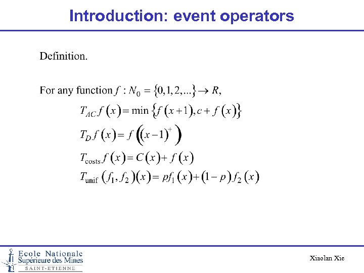Introduction: event operators Xiaolan Xie

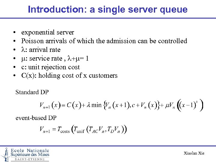Introduction: a single server queue • • • exponential server Poisson arrivals of which the admission can be controlled l: arrival rate m: service rate , l+m= 1 c: unit rejection cost C(x): holding cost of x customers Xiaolan Xie

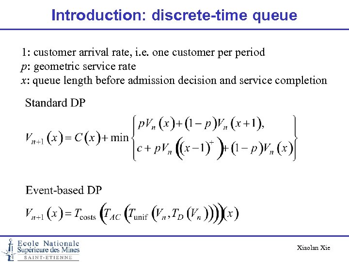Introduction: discrete-time queue 1: customer arrival rate, i. e. one customer period p: geometric service rate x: queue length before admission decision and service completion Xiaolan Xie

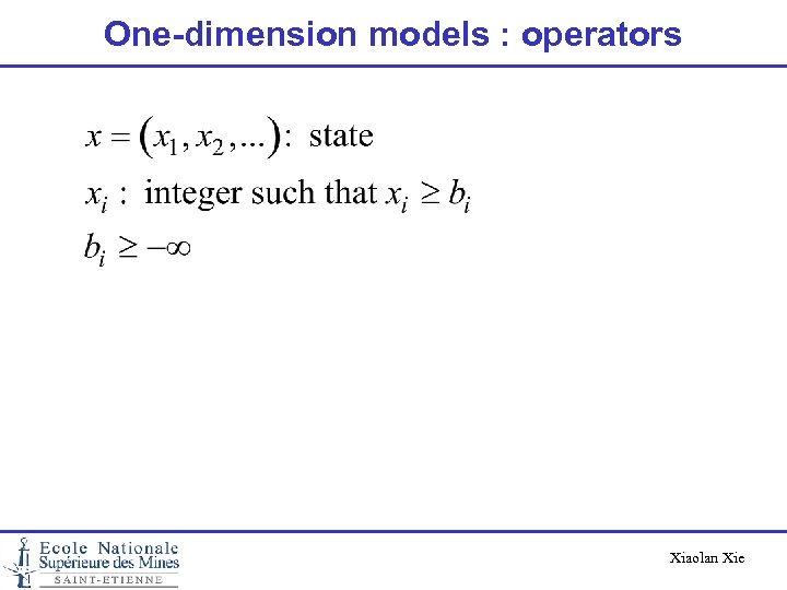One-dimension models : operators Xiaolan Xie

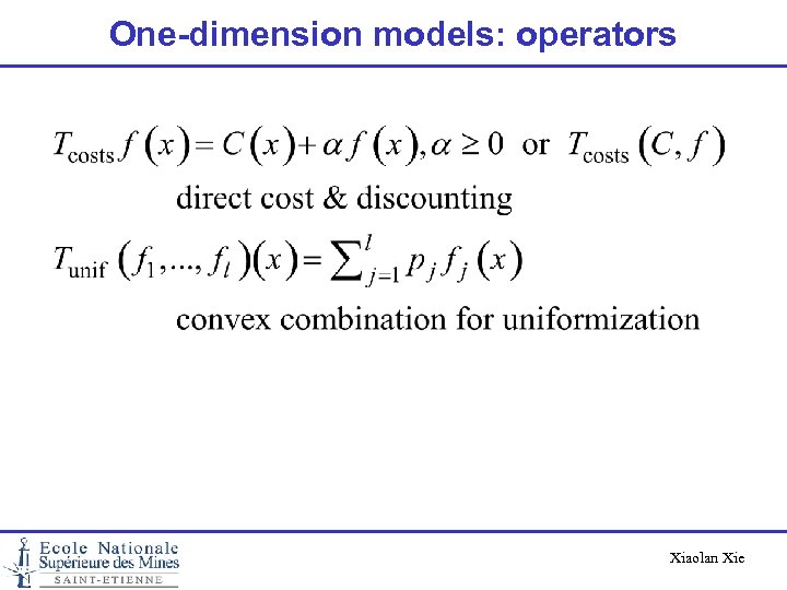One-dimension models: operators Xiaolan Xie

One-dimension models: operators Xiaolan Xie

One-dimension models : operators Xiaolan Xie

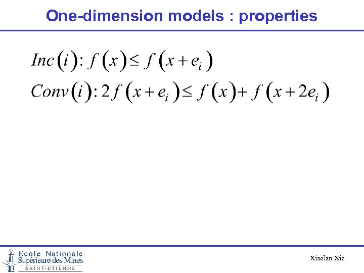One-dimension models : properties Xiaolan Xie

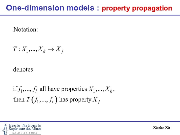One-dimension models : property propagation Xiaolan Xie

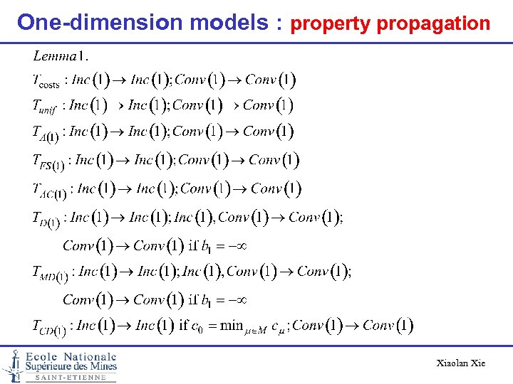One-dimension models : property propagation Xiaolan Xie

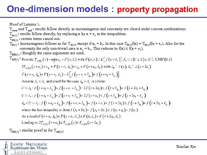One-dimension models : property propagation Proof of Lemma 1. Tcosts and Tunif : results follow directly as increasingness and convexity are closed under convex combinations. TA(1) : results follow directly, by replacing x by x + e 1 in the inequalities. TFS(1) : certain terms cancel out. TD(1) : Increasingness follows as for TA(1), except if x 1 = b 1. In this case TD(1)f(x) = TD(1)f(x + e 1). Also for the convexity the only non-trivial case is x 1 = b 1. This reduces to f(x) f(x + e 1). TMD(1) : Roughly the same arguments are used. TAC(1) : TCD(1) : similar proof as for TAC(1). Xiaolan Xie

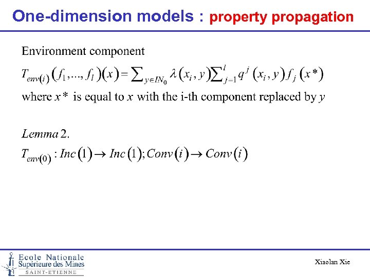One-dimension models : property propagation Xiaolan Xie

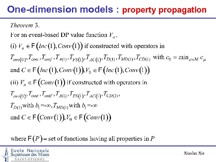One-dimension models : property propagation Xiaolan Xie

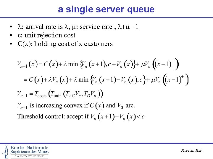a single server queue • l: arrival rate is l, m: service rate , l+m= 1 • c: unit rejection cost • C(x): holding cost of x customers Xiaolan Xie

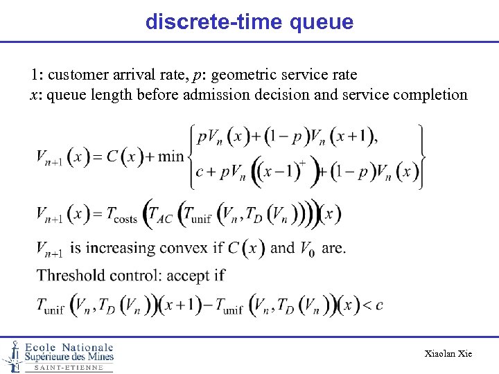discrete-time queue 1: customer arrival rate, p: geometric service rate x: queue length before admission decision and service completion Xiaolan Xie

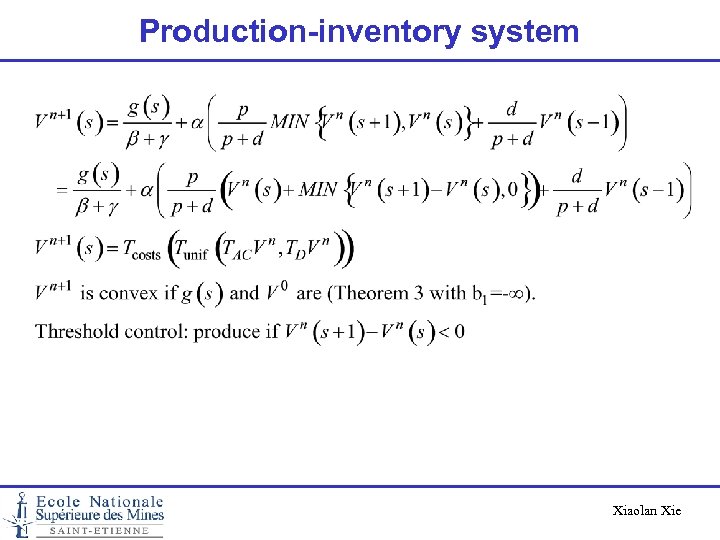Production-inventory system Xiaolan Xie

Multi-machine production-inventory with preemption Xiaolan Xie

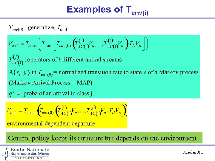Examples of Tenv(i) Control policy keeps its structure but depends on the environment Xiaolan Xie

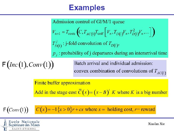Examples Xiaolan Xie

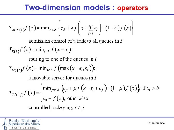Two-dimension models : operators Xiaolan Xie

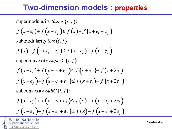Two-dimension models : properties Xiaolan Xie

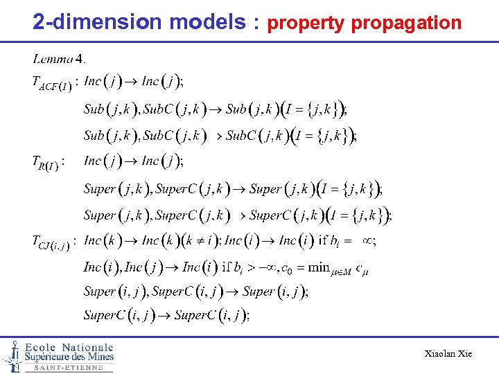
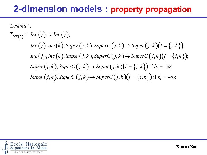
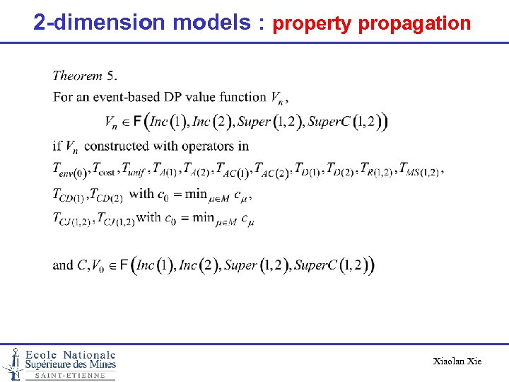
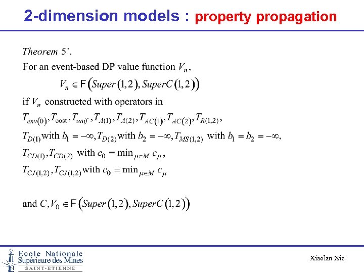
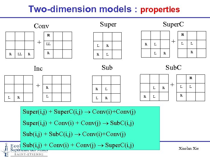Two-dimension models : properties Super Conv Super. C R R + R LL L R R R LL R + L L L R R Sub Inc L Sub. C R + L R R R L L L R L R + L L R Super(i, j) + Super. C(i, j) Conv(i)+Conv(j) Super(i, j) + Conv(i) + Conv(j) Sub. C(i, j) Sub(i, j) + Sub. C(i, j) Conv(i)+Conv(j) Sub(i, j) + Conv(i) + Conv(j) Super. C(i, j) Xiaolan Xie

2 -dimension models : property propagation Xiaolan Xie

2 -dimension models : property propagation Xiaolan Xie

2 -dimension models : property propagation Xiaolan Xie

2 -dimension models : property propagation Xiaolan Xie

2 -dimension models : property propagation Xiaolan Xie

2 -dimension models : property propagation Xiaolan Xie

2 -dimension models : property propagation Xiaolan Xie

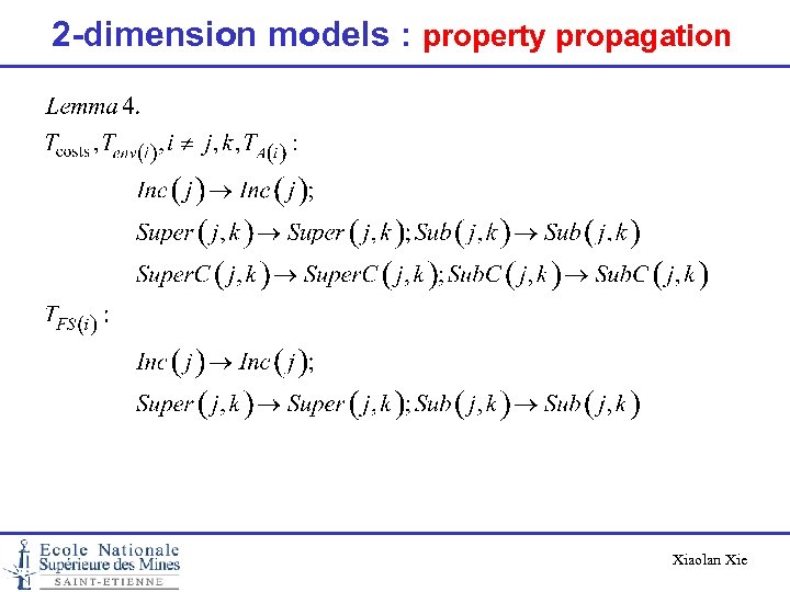
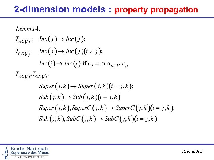
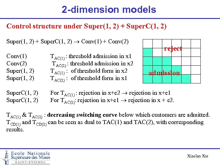2 -dimension models Control structure under Super(1, 2) + Super. C(1, 2) Conv(1) + Conv(2) reject Conv(1) Conv(2) Super(1, 2) TAC(1) : threshold admission in x 1 TAC(2) : threshold admission in x 2 TAC(1) : of threshold form in x 2 TAC(2) : of threshold form in x 1 Super. C(1, 2) For TAC(1) : rejection in x+e 2 rejection in x+e 1 For TAC(2): rejection in x+e 1 rejection in x + e 2. admission TAC(1) & TAC(2) : decreasing switching curve below which customers are admitted. TCD(1) and TCD(2) can be seen as dual to TAC(1) and TAC(2), with corresponding results. Xiaolan Xie

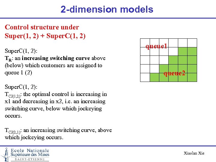2 -dimension models Control structure under Super(1, 2) + Super. C(1, 2): TR: an increasing switching curve above (below) which customers are assigned to queue 1 (2) queue 1 queue 2 Super. C(1, 2): TCJ(1, 2): the optimal control is increasing in x 1 and decreasing in x 2, i. e. an increasing switching curve, below which jockeying occurs. TCJ(2, 1): an increasing switching curve, above which jockeying occurs. Xiaolan Xie

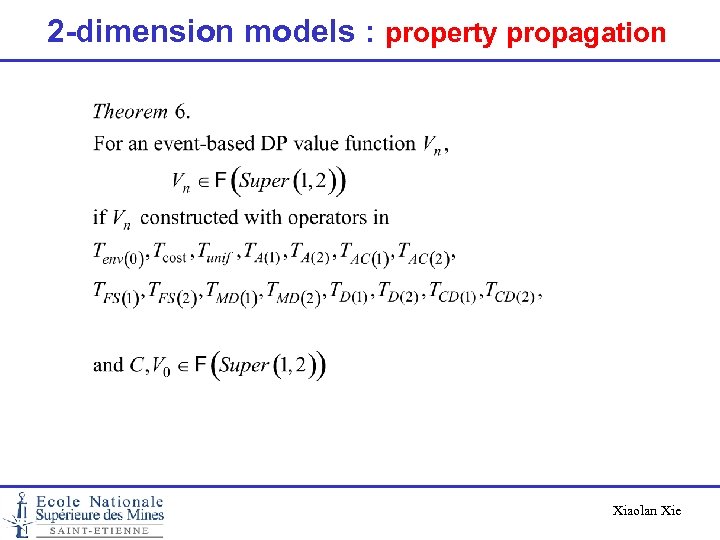2 -dimension models : property propagation Xiaolan Xie

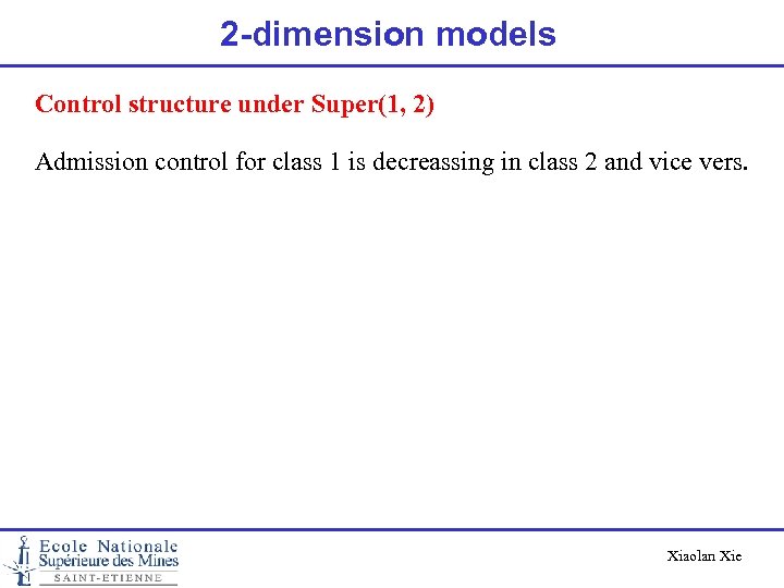2 -dimension models Control structure under Super(1, 2) Admission control for class 1 is decreassing in class 2 and vice vers. Xiaolan Xie

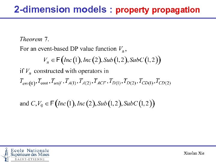2 -dimension models : property propagation Xiaolan Xie

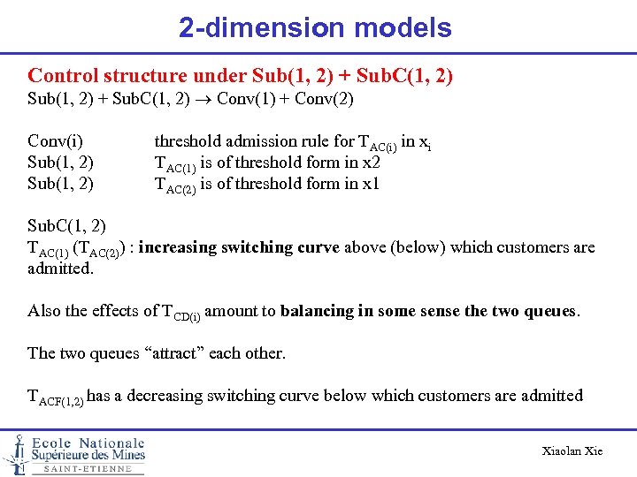2 -dimension models Control structure under Sub(1, 2) + Sub. C(1, 2) Conv(1) + Conv(2) Conv(i) Sub(1, 2) threshold admission rule for TAC(i) in xi TAC(1) is of threshold form in x 2 TAC(2) is of threshold form in x 1 Sub. C(1, 2) TAC(1) (TAC(2)) : increasing switching curve above (below) which customers are admitted. Also the effects of TCD(i) amount to balancing in some sense the two queues. The two queues “attract” each other. TACF(1, 2) has a decreasing switching curve below which customers are admitted Xiaolan Xie

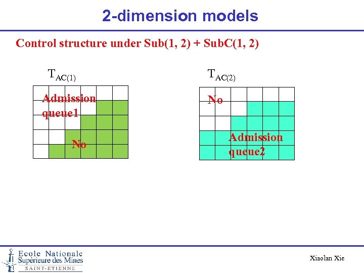2 -dimension models Control structure under Sub(1, 2) + Sub. C(1, 2) TAC(1) Admission queue 1 No TAC(2) No Admission queue 2 Xiaolan Xie

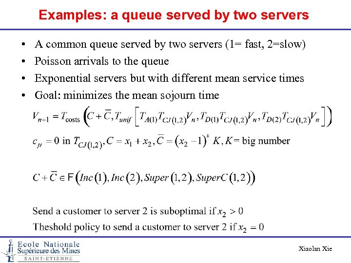Examples: a queue served by two servers • • A common queue served by two servers (1= fast, 2=slow) Poisson arrivals to the queue Exponential servers but with different mean service times Goal: minimizes the mean sojourn time Xiaolan Xie

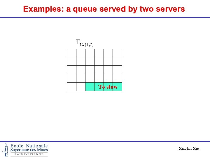Examples: a queue served by two servers TCJ(1, 2) To slow Xiaolan Xie

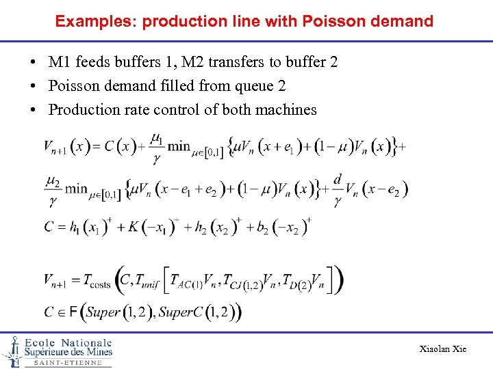Examples: production line with Poisson demand • M 1 feeds buffers 1, M 2 transfers to buffer 2 • Poisson demand filled from queue 2 • Production rate control of both machines Xiaolan Xie

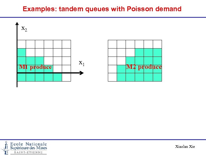Examples: tandem queues with Poisson demand x 2 M 1 produce x 1 M 2 produce Xiaolan Xie

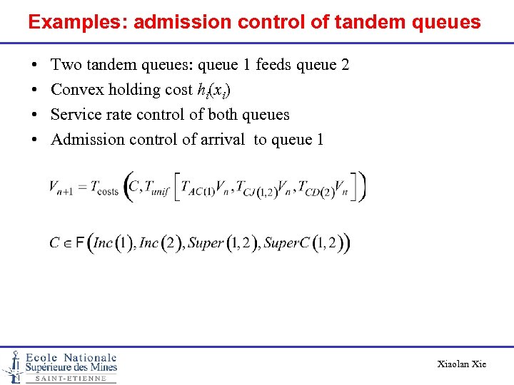Examples: admission control of tandem queues • • Two tandem queues: queue 1 feeds queue 2 Convex holding cost hi(xi) Service rate control of both queues Admission control of arrival to queue 1 Xiaolan Xie

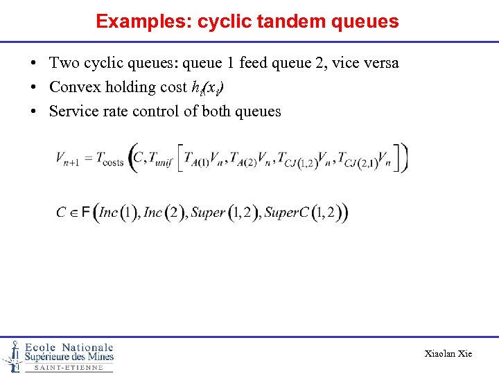Examples: cyclic tandem queues • Two cyclic queues: queue 1 feed queue 2, vice versa • Convex holding cost hi(xi) • Service rate control of both queues Xiaolan Xie

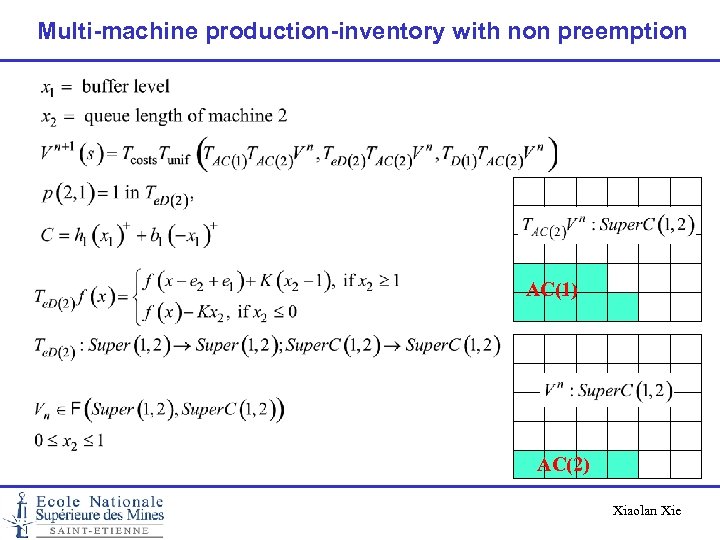Multi-machine production-inventory with non preemption AC(1) AC(2) Xiaolan Xie

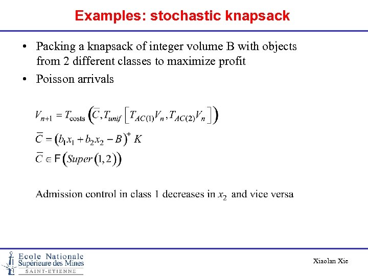Examples: stochastic knapsack • Packing a knapsack of integer volume B with objects from 2 different classes to maximize profit • Poisson arrivals Xiaolan Xie

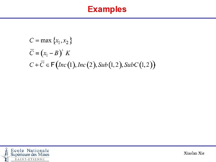Examples Xiaolan Xie