Physical Layer Transmission Media Transmission Media

Physical Layer – Transmission Media

Transmission Media • Two basic formats – Guided media : wires, fiber optics • Medium is important – Unguided media : wireless, radio transmission • Antenna is important • Each have tradeoffs over data rate, distance – Attenuation : weakening of signal over distance

Mini Electromagnetic Review • Take a sound wave… Frequency (hz) = Number of cycles/second With a constant wave velocity, frequency = velocity / wavelength For electromagnetic waves, f = c / w ; c = speed of light

Mini Electromagnetic Review Same principle with electrical waves: Station at 88. 1 FM = 88. 1 Mhz 88100000 = 3. 0 * 10^8 / w w = 3. 0 * 10^8 / 88100000 = 3. 4 meters Time to travel this far is 1/f or 0. 000000011 seconds

Electromagnetic Spectrum

Guided Transmission Media • Twisted Pair • Coaxial cable • Optical fiber Attenuation Coax Twisted Pair 1 Khz 1 Mhz Fiber Optics 1 Ghz Frequency 1 Thz 1000 Thz

Twisted Pair of copper wires constitutes a single communication link. Twists minimize the effects of electromagnetic interference - emit less emag energy - less susceptible to emag energy

Twisted Pair - Applications • Most common medium • Telephone network – POTS – Between house and local exchange (subscriber loop), also called the end office. From the end office to Central Office (CO) class 4 CO class 1 via Public Switched Telephone Network (PSTN) • Within buildings – To private branch exchange (PBX) • For local area networks (LAN) – 10 Mbps or 100 Mbps – Possible to rev up to 1 Gbps – Gigabit Ethernet

Twisted Pair - Pros and Cons • Cheap • Easy to work with – Can use as digital or analog • Limited bandwidth/data rate – Generally 1 Mhz and 100 Mbps but up to 1 Ghz • Short range – 2 km for digital, 5 km for analog • Direct relationship between data rate and range – Gigabit Ethernet • 1000 Mbps over 4 Cat 5 UTP up to 100 meters – IEEE 802. 3 ab standard in 1999 • 1000 Mbps over 1 Cat 5 UTP up to 24 meters

Unshielded and Shielded TP • Unshielded Twisted Pair (UTP) – – Ordinary telephone wire Cheapest Easiest to install Suffers from external EM interference • Shielded Twisted Pair (STP) – Metal braid or sheathing that reduces interference – More expensive – Harder to handle (thick, heavy)

UTP Categories • Cat 1 – Used for audio frequencies, speaker wire, etc. Not for networking. • Cat 2 – Up to 1. 5 Mhz, used for analog phones, not for networking • Cat 3 – EIA 568 -A Spec from here on up – up to 16 MHz – Voice grade once common in offices, 10 Mb networks – Twist length of 7. 5 cm to 10 cm • Cat 4 – up to 20 MHz – Not frequently used today, was used for Token Ring

UTP Categories Cont. • Cat 5 – up to 100 MHz – Twist length 0. 6 cm to 0. 85 cm – Commonly pre-installed in new office buildings • Cat 5 e “Enhanced” – Up to 100 Mhz – Specifies minimum characteristics for NEXT (Near End Crosstalk) and ELFEXT (Equal level far end crosstalk) • Coupling of signal from one pair to another • Coupling takes place when transmit signal entering the link couples back to receiving pair, i. e. near transmitted signal is picked up by near receiving pair • Cat 6 – Standard up to 250 Mhz; heavier, up to 100 meters • Cat 6 a – Standard up to 500 Mhz

Typical Usage of Twisted Pair Name Cat 1 Type UTP Mbps 1 m 90 In… Cat 2 UTP 4 90 Tkn Ring/Phone Cat 3 UTP 10 10 Base. T Cat 4 STP 16 100 TRing 16 Cat 5 S/UTP Cat 6 S/UTP 100 to 200 10 Gbps 100 Base. T & 1000 Base. T 10 GBase. T

Coaxial Cable Shielded, less susceptible to noise and attenuation than Twisted Pair.

Coaxial Cable Applications • Most versatile medium • Television distribution – Cable TV • Long distance telephone transmission – Can carry 10, 000 voice calls simultaneously – Being replaced by fiber optic • Short distance computer systems links • Local area networks – More expensive than twisted pair, not as popular for LANs

Coaxial Cable Characteristics • Analog – Broadband Coaxial Cable – Amplifiers every few km, closer if higher frequency – Up to 500 MHz – Cable TV, Cable Modems (~10 Mbps) • Digital – Baseband Coaxial Cable – Repeater every 1 km – Closer for higher data rates Name Type Mbps m In… RG-58 Coax 10 185 10 Base 2, “Thin. Net” RG-8 Coax 10 500 10 Base 5, “Thick. Net”

Coaxial Cable LAN

Optical Fiber Breakthrough in data transmission systems! Core: Thin strands of glass Cladding: Glass with different optical properties than core Jacket: Plastic/Insulation

Optical Fiber - Benefits • Greater capacity – Data rates of hundreds of Gbps – Tbps demonstrated using WDM • Smaller size & weight – Order of magnitude smaller than TP/Coax • Lower attenuation • Electromagnetic isolation – Not vulnerable to interference, impulse, crosstalk! • Greater repeater spacing – Often 10’s of kilometers • Hard to tap

Optical Fiber Transmission Modes Rays at shallow angles reflect; multiple propagation path spreads signal out over time Gradient refraction in core allows light to curve helically, more coherent at end Shrink core to allow only a single angle or mode, light reflect in only one pattern

Wireless or Radiated Transmission • Unguided media • Transmission and reception via antenna – Desirable to make antenna one-quarter or one-half the wavelength • Directional – Focused beam – Careful alignment required • Omnidirectional – Signal spreads in all directions – Can be received by many antennas

Frequencies • 2 GHz to 40 GHz – – Microwave Highly directional Point to point Satellite • 30 MHz to 1 GHz – Omnidirectional – Broadcast radio • 3 x 1011 to 2 x 1014 – Infrared – Local • Higher frequencies Higher data rates

Terrestrial Microwave • Typically parabolic dish, focused beam, line of sight • Max distance between antenna: d=7. 14 * Sqrt(h. K) ; K=4/3, ; h=antenna ht in meters ; d=distance in km so two 1 meter antenna can be 7. 14*Sqrt(4/3)=8. 2 km apart • Applications – Long haul telecommunications, television. May need repeaters – Short range for BN or closed-circuit TV

Terrestrial Microwave • Data rate increases with frequency – 2 Ghz Band 7 Mhz Bandwidth 12 Mbps – 6 Ghz Band 30 Mhz Bandwidth 90 Mbps – 11 Ghz Band 40 Mhz Bandwidth 135 Mbps – 18 Ghz Band 220 Mhz Bandwidth 274 Mbps • Attenuation – Loss varies with the square of the distance – TP/Coax: loss varies with log of distance / linear in d. B – Therefore, we don’t need as many repeaters with microwave • Interference and Raindrop Attenuation – Frequency bands strictly regulated – Use lower frequency to avoid raindrop problem

Satellite Microwave • Satellite is relay station • Satellite receives on one frequency, amplifies or repeats signal and transmits on another frequency/frequencies (transponder channels) • Typically geo-stationary orbit – Height of 35, 784 km or 22, 236 miles – 4 degree spacing in 4/6 Ghz Band – 3 degree spacing in 12/14 Ghz Band • Applications – TV, telephone – Private business networks – VSAT (Very Small Aperture Terminal) • Large corp. with distributed sites • Small receiver to Ku-band satellite to Big earth hub • Used by RCA in late 1994 for Direct Broadcast System

Satellite Transmission Characteristics • Optimum Frequency Range 1 -10 Ghz – Below 1 Ghz, natural noise. Above 10 Ghz, attenuation from the atmosphere – Most applications use the 5. 925 -6. 425 Ghz range uplink, 4. 2 -4. 7 Ghz range downlink (4/6 Ghz Band) • Propagation delay – 35784000 m / 3. 0 * 108 m/s 0. 12 seconds one way – About quarter second propagation delay round trip, noticeable for phone conversations, problem for twoway communications • Error /flow control? • Low orbit satellites a solution? (Iridium, Tachyon)

Broadcast Radio • 30 Mhz to 2 Ghz • Omnidirectional – Use loop or wire antenna instead of dish • Applications – Range covers FM radio, UHF and VHF television – 802. 11 b operates in the 2. 4 Ghz ISM band • Due to lower frequencies than microwave, less problems with attenuation • Same equation for antenna distance, attenuation as microwave • Drawbacks – Suffers from multipath interference, Reflections – Possible security concerns

Infrared • • Modulate noncoherent infrared light Line of sight (or reflection) Blocked by walls Problems – Short range, usually 50 -75 feet maximum – Low speed, 1 -4 Mbps • e. g. TV remote control, IRD port – For networks, not generally used due to the need for direct line-of-sight; was used to connect hubs

Media Selection Guided Media Network Type Cost Transmission Distance Error Security Rates Speed Twisted Pair Coaxial Cable Fiber Optics LAN any Short-Mod Mod. -long Good Low V. Good V. Low-high High-V. High Low Mod. High Radiated Media Network Type Cost Transmission Distance Security Error Rates Radio Infrared Microwave Satellite LAN Low LAN, BN Low WAN Mod Short Long Mod Low Low-Mod Mod Poor Speed

Carriers and Modulation First, review of digital transmission of digital data

Baseband Transmission Digital transmission is the transmission of electrical pulses. Digital information is binary in nature in that it has only two possible states 1 or 0. Sequences of bits encode data (e. g. , text characters). Digital signals are commonly referred to as baseband signals. In order to successfully send and receive a message, both the sender and receiver have to agree how often the sender can transmit data (data rate). Data rate often called bandwidth – but there is a different definition of bandwidth referring to the frequency range of a signal!

Baseband Transmission With unipolar signaling techniques, the voltage is always positive or negative (like a dc current). In bipolar signaling, the 1’s and 0’s vary from a plus voltage to a minus voltage (like an ac current). In general, bipolar signaling experiences fewer errors than unipolar signaling because the signals are more distinct.

Baseband Transmission

Baseband Transmission Manchester encoding is a special type of unipolar signaling in which the signal is changed from a high to low (0) or low to high (1) in the middle of the signal. • More reliable detection of transition rather than level – consider perhaps some constant amount of dc noise, transitions still detectable but dc component could throw off NRZ-L scheme – Transitions still detectable even if polarity reversed Manchester encoding is commonly used in local area networks (ethernet, token ring).

Manchester Encoding

ANALOG TRANSMISSION OF DIGITAL DATA Analog Transmission occurs when the signal sent over the transmission media continuously varies from one state to another in a wave-like pattern. e. g. telephone networks, originally built for human speech rather than data. Advantage for long distance communications: much less attenuation for analog carrier than digital

Digital Data to Analog Transmission Before we get further into Analog to Digital, we need to understand various characteristics of analog transmission.

Periodic Signals

Sine Wave • Peak Amplitude (A) – maximum strength of signal – volts • Frequency (f) – – Rate of change of signal Hertz (Hz) or cycles per second Period = time for one repetition (T) T = 1/f • Phase ( ) – Relative position in time, from 0 -2*pi • General Sine wave

Varying Sine Waves

Wavelength • Distance occupied by one cycle • Distance between two points of corresponding phase in two consecutive cycles • = Wavelength • Assuming signal velocity v – = v. T – f = v – c = 3*108 ms-1 (speed of light in free space)

Frequency Domain Concepts • Signal usually made up of many frequencies • Components are sine (or cosine) waves • Can be shown (Fourier analysis) that any continuous signal is made up of component sine waves • Can plot frequency domain functions

Addition of Frequency Components Notes: 2 nd freq a multiple of 1 st called fundamental freq Others called harmonics Period of combined = Period of the fundamental Fundamental = carrier freq

Frequency Domain Discrete Freq Rep: Any continuous signal can be represented as the sum of sine waves! (May need an infinite number. . ) Discrete signals result in Continuous, Infinite Frequency Rep: s(t)=1 from –X/2 to X/2

Data Rate and Bandwidth • Any transmission system has a limited band of frequencies • This limits the data rate that can be carried • Spectrum – range of frequencies contained in signal • Absolute bandwidth – width of spectrum • Effective bandwidth – Often just bandwidth – Narrow band of frequencies containing most of the energy

Example of Data Rate/Bandwidth Want to transmit: Let’s say that f=1 Mhz or 106 cycles/second, so T= 1 microsecond Let’s approximate the square wave with a few sine waves:

Ex(1): Sine Wave 1 Bandwidth=5 f-f =4 f If f=1 Mhz, then the bandwidth = 4 Mhz T=1 microsecond; we can send two bits per microsecond so the data rate = 2 * 106 = 2 Mbps

Ex(2): Sine Wave 1, Higher freq Bandwidth=5 f-f =4 f If f=2 Mhz, then the bandwidth = 8 Mhz T=0. 5 microsecond; we can send two bits per 0. 5 microseconds or 4 bits per microsecond, so the data rate = 4 * 106 = 4 Mbps Double the bandwidth, double the data rate!

Ex(3): Sine Wave 2 Bandwidth=3 f-f =2 f If f=2 Mhz, then the bandwidth = 4 Mhz T=0. 5 microsecond; we can send two bits per 0. 5 microseconds or 4 bits per microsecond, so the data rate = 4 * 106 = 4 Mbps Still possible to get 4 Mbps with the “lower” bandwidth, but our receiver must be able to discriminate from more distortion!

Bandwidth / Representation 2000 bps B=500 Hz B=1000 Hz B=1700 Hz B=4000 Hz Increasing bandwidth improves the representation of the data signal. 500 Hz too low to reproduce the signal. Want to maximize the capacity of the available bandwidth.

Frequency Division Multiplexing (FDM)

Time Division Multiplexing (TDM)

Transmission Impairments • Signal received may differ from signal transmitted • Analog - degradation of signal quality • Digital - bit errors • Caused by – Attenuation and attenuation distortion – Delay distortion – Noise

Attenuation • Signal strength falls off with distance • Depends on medium • Received signal strength: – must be enough to be detected – must be sufficiently higher than noise to be received without error • Attenuation is an increasing function of frequency; higher frequencies suffer from more attenuation. Can distort the signal. • Solution: Equalization. Boost higher frequency components.

Delay Distortion • Only in guided media • Propagation velocity varies with frequency – Velocity highest near center frequency – Results in phase shift at different frequencies – “Overlapping” bits • Solution: Equalization

Noise (1) • Additional signals inserted between transmitter and receiver • Thermal – Due to thermal agitation of electrons – Uniformly distributed – White noise • Intermodulation – Signals that are the sum and difference of original frequencies sharing a medium

Noise (2) • Crosstalk – A signal from one line is picked up by another • Impulse – Irregular pulses or spikes – e. g. External electromagnetic interference – Short duration – High amplitude

What Causes Errors? Summary of Errors and Noise: Source of Error Line Outages White Noise Impulse Noise Cross-Talk Echo Attenuation What Causes It Storms, Accidents Movement of electrons Sudden increases in electricity (e. g. lightning) Multiplexer guardbands too small, or wires too close together Poor connections How to Prevent It. Increase signal strength Shield or move the wires Increase the guardbands, or move or shield the wires Fix the connections, or tune equipment Use repeaters or amps Graduate decrease in signal over distance Signals from several circuits combine Move or shield the wires Intermodulation Noise Analog signals change phase Jitter Harmonic Distortion Amplifier changes phase Tune equipment

Error Prevention There are many ways to prevent errors: • Shielding (adding insulation) • Moving cables away from noise sources • Changing multiplexing type (FDM TDM) • Tuning transmission equipment and improving connection quality • Using amplifiers and repeaters • Equalization

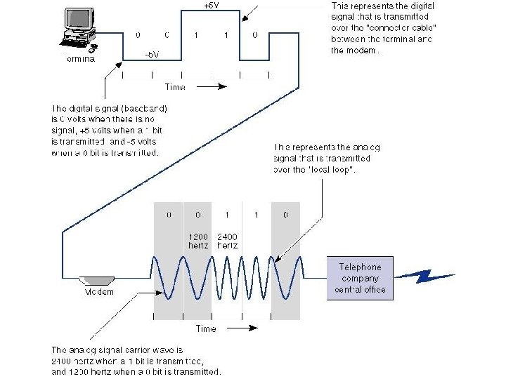
Modulation - Digital Data, Analog Signal • Public telephone system – 300 Hz to 3400 Hz • Guardband from 0 -300, 3400 -4000 Hz – Use modem (modulator-demodulator) • Amplitude shift keying (ASK) • Frequency shift keying (FSK) • Phase shift keying (PSK)

Amplitude Modulation and ASK

Frequency Modulation and FSK

Phase Modulation and PSK

Amplitude Shift Keying • Values represented by different amplitudes of carrier • Usually, one amplitude is zero – i. e. presence and absence of carrier is used • • Susceptible to sudden gain changes Inefficient Typically used up to 1200 bps on voice grade lines Used over optical fiber

Frequency Shift Keying • Values represented by different frequencies (near carrier) • Less susceptible to error than ASK • Typically used up to 1200 bps on voice grade lines • High frequency radio • Even higher frequency on LANs using coax

FSK on Voice Grade Line Bell Systems 108 modem

Phase Shift Keying • Phase of carrier signal is shifted to represent data • Differential PSK – Phase shifted relative to previous transmission rather than some reference signal

Sending Multiple Bits Simultaneously Each of the three modulation techniques can be refined to send more than one bit at a time. It is possible to send two bits on one wave by defining four different amplitudes. This technique could be further refined to send three bits at the same time by defining 8 different amplitude levels or four bits by defining 16, etc. The same approach can be used for frequency and phase modulation.

Sending Multiple Bits Simultaneously

Sending Multiple Bits Simultaneously In practice, the maximum number of bits that can be sent with any one of these techniques is about five bits. The solution is to combine modulation techniques. One popular technique is quadrature amplitude modulation (QAM) involves splitting the signal into eight different phases, and two different amplitude for a total of 16 different possible values, giving us lg(16) or 4 bits per value.

2 -D Diagram of QAM

Sending Multiple Bits Simultaneously Trellis coded modulation (TCM) is an enhancement of QAM that combines phase modulation and amplitude modulation. The problem with high speed modulation techniques such as TCM is that they are more sensitive to imperfections in the communications circuit.

Bits Rate Versus Baud Rate Versus Symbol Rate The terms bit rate (the number of bits per second) and baud rate are used incorrectly much of the time. They are not the same. A bit is a unit of information, a baud is a unit of signaling speed, the number of times a signal on a communications circuit changes. ITU-T now recommends the term baud rate be replaced by the term symbol rate.

Bits Rate Versus Baud Rate Versus Symbol Rate The bit rate and the symbol rate (or baud rate) are the same only when one bit is sent on each symbol. If we use QAM or TCM, the bit rate would be several times the baud rate. Typically we use compression techniques on top of the modulation technique

Analog Data, Digital Signal • Digitization – Conversion of analog data into digital data – Digital data can then be transmitted using digital signaling (e. g. Manchester) – Or, digital data can then be converted to analog signal – Analog to digital conversion done using a codec (coder/decoder) – Two techniques to convert analog to digital • Pulse code modulation / Pulse amplitude modulation • Delta modulation

Pulse Amplitude Modulation Analog voice data must be translated into a series of binary digits before they can be transmitted. With Pulse Amplitude Modulation, the amplitude of the sound wave is sampled at regular intervals and translated into a binary number. The difference between the original analog signal and the translated digital signal is called quantizing error.

Pulse Amplitude Modulation

Pulse Amplitude Modulation

Pulse Amplitude Modulation

Pulse Amplitude Modulation For standard voice grade circuits, the sampling of 3300 Hz at an average of 2 samples/second would result in a sample rate of 6600 times per second. There are two ways to reduce quantizing error and improve the quality of the PAM signal. – Increase the number of amplitude levels – Sample more frequently (oversampling).

Pulse Code Modulation is the most commonly used technique in the PAM family and uses a sampling rate of 8000 samples per second. Each sample is an 8 bit sample resulting in a digital rate of 64, 000 bps (8 x 8000). Sampling Theorem: If a signal is sampled at a rate higher than twice the highest signal frequency, then the samples contain all the information of the original signal. E. g. : For voice capped at 4 Khz, can sample at 8000 times per second to regenerate the original signal.

Performance of A/D techniques • Good voice reproduction via PCM – PCM - 128 levels (7 bit) – Voice bandwidth 4 khz – Should be 8000 x 7 = 56 kbps for PCM • (Actually 8000 x 8 with control bit) • Data compression can improve on this – e. g. Interframe coding techniques for video • Why digital? – Repeaters instead of amplifiers; don’t amplify noise – Allows efficient and flexible Time Division Multiplexing over Frequency Division Multiplexing – Conversion to digital allows use of more efficient digital switching techniques