PHITS Multi-Purpose Particle and Heavy Ion Transport code

PHITS Multi-Purpose Particle and Heavy Ion Transport code System Exercises using Recommendation Settings and Utilities Jun. 2013 revised title 1

Contents • Recommendation Settings • Particle. Therapy • H 10 mupliplier • Utilities • Animation of Particle Trajectories • Simple. GEO • Summary and Homework Contents 2

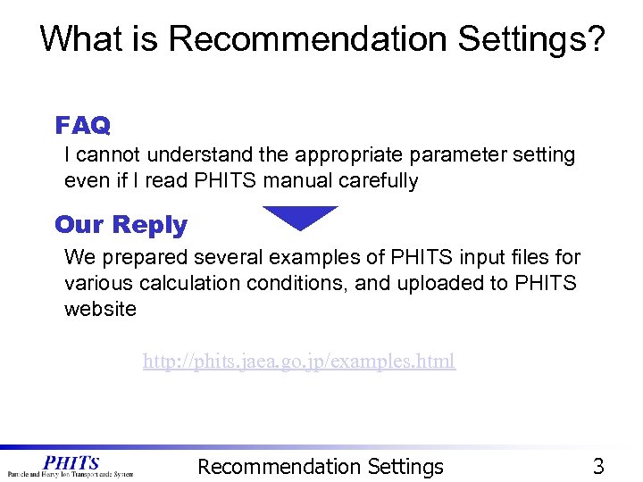What is Recommendation Settings? FAQ I cannot understand the appropriate parameter setting even if I read PHITS manual carefully Our Reply We prepared several examples of PHITS input files for various calculation conditions, and uploaded to PHITS website http: //phits. jaea. go. jp/examples. html Recommendation Settings 3

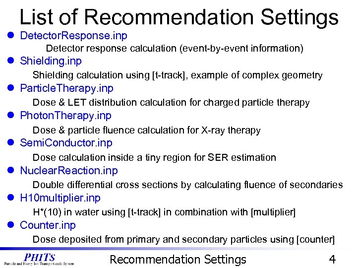List of Recommendation Settings l Detector. Response. inp 　　　　Detector response calculation (event-by-event information) l Shielding. inp Shielding calculation using [t-track], example of complex geometry l Particle. Therapy. inp Dose & LET distribution calculation for charged particle therapy l Photon. Therapy. inp Dose & particle fluence calculation for X-ray therapy l Semi. Conductor. inp Dose calculation inside a tiny region for SER estimation l Nuclear. Reaction. inp Double differential cross sections by calculating fluence of secondaries l H 10 multiplier. inp H*(10) in water using [t-track] in combination with [multiplier] l Counter. inp Dose deposited from primary and secondary particles using [counter] Recommendation Settings 4

Contents • Recommendation Settings • Particle. Therapy • H 10 mupliplier • Utilities • Animation of Particle Trajectories • Simple. GEO • Summary and Homework Contents 5

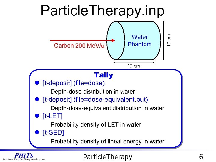Carbon 200 Me. V/u Water Phantom 10 cm Particle. Therapy. inp 10 cm Tally l [t-deposit] (file=dose) Depth-dose distribution in water l [t-deposit] (file=dose-equivalent. out) Depth-dose-equivalent distribution in water l [t-LET] Probability density of LET in water l [t-SED] Probability density of lineal energy in water Particle. Therapy 6

Dose and Dose Equivalent Dose. eps [ T - Deposit ] mesh = r-z r-type = 2 rmin = 0. 000000 rmax = 1. 000000 nr = 1 z-type = 2 zmin = 0. 000000 zmax = 10. 00000 nz = 100 dedxfnc = 0 Dose-equivalent. eps [ T - Deposit ] dedxfnc = 1 R Output quantities are weighted by the function written in usrdfn 1. f Z r-z mesh Q(L) relationship is given as default Dose is converted into Dose equivalent! Particle. Therapy 7

Probability Density of LET & y [T-LET] [T-SED] LET-distribution. eps (page 1: front surface) y-distribution. eps (page 1: front surface) LET of C(200 Me. V/u) = 16 ke. V/mm L*f(L) has Sharp peak y*f(y) broad distribution even for mono-energetic incidence Particle. Therapy 8

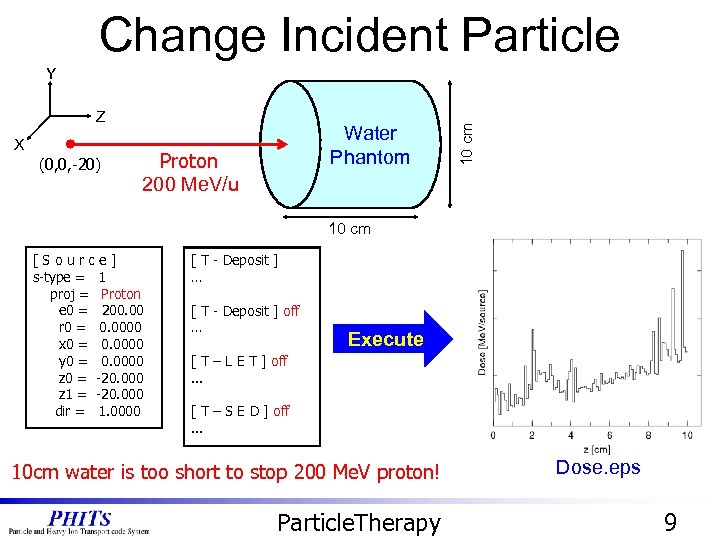Change Incident Particle Z X (0, 0, -20) Water Phantom Carbon Proton 200 Me. V/u 10 cm Y 10 cm [Source] s-type = 1 proj = 12 C Proton e 0 = 200. 00 r 0 = 0. 0000 x 0 = 0. 0000 y 0 = 0. 0000 z 0 = -20. 000 z 1 = -20. 000 dir = 1. 0000 [ T - Deposit ] … [ T - Deposit ] off … Execute [ T – L E T ] off. . . [ T – S E D ] off. . . 10 cm water is too short to stop 200 Me. V proton! Particle. Therapy Dose. eps 9

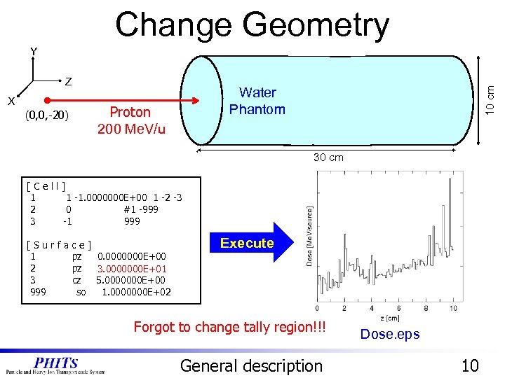Change Geometry X (0, 0, -20) Water Phantom Carbon Proton 200 Me. V/u 10 cm Z 10 cm Y 30 cm [Cell] 1 1 -1. 0000000 E+00 1 -2 -3 2 0 #1 -999 3 -1 999 [Surface] 1 pz 0. 0000000 E+00 2 pz 1. 0000000 E+01 3 cz 5. 0000000 E+00 999 so 1. 0000000 E+02 Execute Forgot to change tally region!!! General description Dose. eps 10

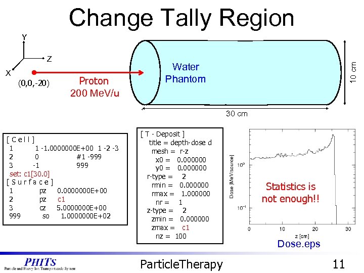Change Tally Region X (0, 0, -20) Carbon Proton 200 Me. V/u Water Phantom 10 cm Z 10 cm Y 30 cm [Cell] 1 1 -1. 0000000 E+00 1 -2 -3 2 0 #1 -999 3 -1 999 set: c 1[30. 0] [Surface] 1 pz 0. 0000000 E+00 c 1 2 pz 2. 0000000 E+01 3 cz 5. 0000000 E+00 999 so 1. 0000000 E+02 [ T - Deposit ] title = depth-dose d mesh = r-z x 0 = 0. 000000 y 0 = 0. 000000 r-type = 2 rmin = 0. 000000 rmax = 1. 000000 nr = 1 z-type = 2 zmin = 0. 000000 zmax = 10. 00000 c 1 nz = 100 Particle. Therapy Statistics is not enough!! Dose. eps 11

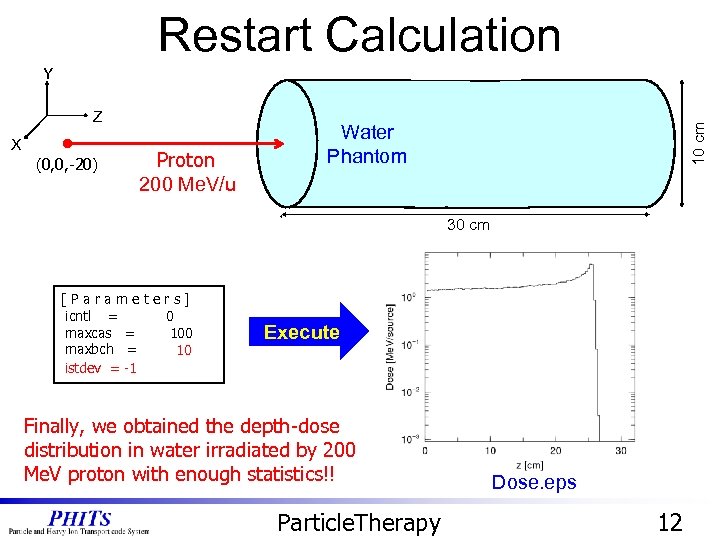Restart Calculation X (0, 0, -20) Carbon Proton 200 Me. V/u Water Phantom 10 cm Z 10 cm Y 30 cm [Parameters] icntl = 0 maxcas = 100 maxbch = 　2 10 istdev = -1 Execute Finally, we obtained the depth-dose distribution in water irradiated by 200 Me. V proton with enough statistics!! Particle. Therapy Dose. eps 12

Contents • Recommendation Settings • Particle. Therapy • H 10 mupliplier • Utilities • Animation of Particle Trajectories • Simple. GEO • Summary and Homework Contents 13

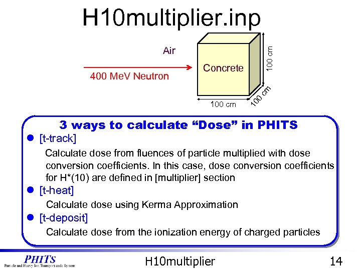H 10 multiplier. inp Concrete 10 100 cm 400 Me. V Neutron 100 cm Air 3 ways to calculate “Dose” in PHITS l [t-track] Calculate dose from fluences of particle multiplied with dose conversion coefficients. In this case, dose conversion coefficients for H*(10) are defined in [multiplier] section l [t-heat] Calculate dose using Kerma Approximation　　 l [t-deposit] Calculate dose from the ionization energy of charged particles H 10 multiplier 14

Results of Each Tally [T-Track] [T-Heat] [T-Deposit] l [t-track] Fluence multiplied with H*(10) dose conversion coefficients 　　→ No gap between concrete and air l [t-heat] Kerma approximation for low-energy neutrons and photons 　　　→There is a gap between concrete and air l [t-deposit] Ionizing energy of charged particles 　　　 → There is a gap between concrete and air. Large uncertainties in air H 10 multiplier 15

Calculation of H*(10) and Effective Dose Fluence calculated by [t-track] can be multiplied with several functions that are pre-defined or defined in [multiplier] section [ Multiplier ] number = -250 interpolation = log ne = 140 1. 13000 E-08 9. 14000 E+00*3600*1. 0 e-6 1. 42000 E-08 9. 44000 E+00*3600*1. 0 e-6 1. 79000 E-08 9. 83000 E+00*3600*1. 0 e-6. . . [T-Track] title = H*(10) in xyz mesh in u. Sv/h. . . multiplier = all part = neutron emax = 1000. 0 mat mset 1 　mset 2 all ( 1. 0 -250 ) (1. 0 -102) multiplier = all part = photon emax = 1000. 0 mat mset 1 mset 2 all ( 1. 0 -251) (1. 0 -114) H*(10) Effective Dose (Page 1) (Page 2) Track. eps They seem to be almost the same! • • H*(10) conversion coefficient for neutron(-250) and photon (-251) defined in [multiplier] Predefined Effective dose conversion coefficients for neutron (-102) and photon (-114) H 10 multiplier 16

Change Axis [T-Track] title = H*(10) in xy part = ( neutron photon ) mesh = xyz x-type = 2 xmin = -60. 0 xmax = 60. 0 Execute nx = 60 1 y-type = 2 ymin = -60. 0 ymax = 60. 0 ny = 1 z-type = 2 Avoid to output zmin = 0. 0 too much graphs zmax = 120. 0 nz = 60 e-type = 1 ne = 1 1. 00000 E-10 1. 00000 E+03 unit = 1 material = all 2 D-plot (contour map) to z axis = xz 1 D-plot (histogram) file = track. out H*(10) Effective Dose (Page 1) (Page 2) Track. eps Tough to compare because each scale is automatically adjusted H 10 multiplier 17

Adjust Scale [T-Track] title = H*(10) in xy part = ( neutron photon ) mesh = xyz x-type = 2 xmin = -60. 0 xmax = 60. 0 Execute 1 nx = 60 y-type = 2 ymin = -60. 0 ymax = 60. 0 ny = 1 z-type = 2 zmin = 0. 0 zmax = 120. 0 nz = 60 e-type = 1 ne = 1 1. 00000 E-10 1. 00000 E+03 unit = 1 material = all z axis = xz file = track. out angel = ymin(5. e-05) ymax(5. e-4) H*(10) Effective Dose (Page 1) (Page 2) Track. eps H*(10) < Effective dose Add ANGEL parameter (min & max for y-axis) H 10 multiplier 18

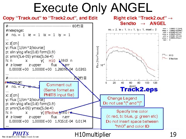Execute Only ANGEL Copy “Track. out” to “Track 2. out”, and Edit #------------------------ 80行目 #newpage: # no. = 1 ie = 1 ix = 1 iy = 1 … x: z[cm] y: Flux [1/cm^2/source] p: xlin ylog afac(0. 8) form(0. 9) p: ymin(5. e-05) ymax(5. 0 e-4) h: n x y(p 1 -group), hh 0 l n H 10 # z-lower z-upper flux r. err 0. 0000 E+00 1. 2809 E-04 0. 0263 … #------------------------- 232行目 #newpage: # no. = 2 ie = 1 ix Comment out = 1 iy = 1 (Same format as … PHITS input file) x: z[cm] y: Flux [1/cm^2/source] p: xlin ylog afac(0. 8) form(0. 9) p: ymin(5. e-05) ymax(5. 0 e-4) h: n x y(p 1 -group), hh 0 lr n Effective # z-lower z-upper flux r. err 0. 0000 E+00 1. 9351 E-04 0. 0174. . . Right click “Track 2. out” →　 Sendto　→　ANGEL Track 2. eps Change Legend Do not use “(“ and “)” Specify line color (r: red, b: blue, g: green etc) Do not insert space between “hh 0 l” and color ID H 10 multiplier 19

Contributions from High- and Low-Energy Particles [T-Track] title = H*(10) in xy part = ( neutron photon ) mesh = xyz x-type = 2 xmin = -60. 0 xmax = 60. 0 Execute nx = 1 y-type = 2 ymin = -60. 0 ymax = 60. 0 ny = 1 z-type = 2 zmin = 0. 0 zmax = 120. 0 nz = 60 e-type = 1 ne = 12 1. 00000 E-10 1. 00000 E+03 20. 0 1. 0 E+03 unit = 1 Divide the energy bin material = all into high- and lowaxis = z energy region file = track. out angel = ymin(1. e-05) ymax(2. e-4) Low Energy (page 1) Low Energy (page 3) ≅ High Energy (page 2) High Energy (page 4) < H*(10) H 10 multiplier Effective Dose 20

Contents • Recommendation Settings • Particle. Therapy • H 10 mupliplier • Utilities • Animation of Particle Trajectories • Simple. GEO • Summary and Homework Contents 21

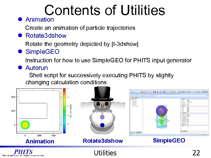Contents of Utilities l Animation Create an animation of particle trajectories l Rotate 3 dshow Rotate the geometry depicted by [t-3 dshow] l Simple. GEO Instruction for how to use Simple. GEO for PHITS input generator l Autorun 　　Shell script for successively executing PHITS by slightly changing calculation conditions Animation Rotate 3 dshow Utilities Simple. GEO 22

Contents • Recommendation Settings • Particle. Therapy • H 10 mupliplier • Utilities • Animation of Particle Trajectories • Simple. GEO • Summary and Homework Contents 23

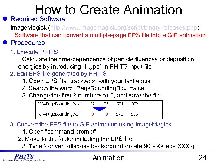How to Create Animation l Required Software Image. Magick (http: //www. imagemagick. org/script/binary-releases. php) 　　Software that can convert a multiple-page EPS file into a GIF animation l Procedures 1. Execute PHITS 　　Calculate the time-dependence of particle fluences or deposition energies by introducing “t-type” in PHITS input file 2. Edit EPS file generated by PHITS 　　1. Open EPS file “track. eps” with your text editor 　　2. Search the word “Page. Bounding. Box” twice 　　3. Change the first 2 numbers to 0, and save the file %%Page. Bounding. Box: 27 36 571 803 %%Page. Bounding. Box: 0 0 571 803 3. Convert the EPS file to GIF animation using Image. Magick 　　1. Open “command prompt” 2. Move to the folder including the EPS file 　　3. Type ‘convert -dispose background -rotate 90 XXX. eps XXX. gif‘ Animation 24

Increase the Time Resolution animation. inp [T-Track] C -- Contour figure Tally -mesh = xyz. . . t-type = 2 nt = 20 # Number of frame 60 tmin = 0. 00 # Initial time (nsec) tmax = 40 # Final time (nsec). . . angel = cmin(1. e-05) cmax(1. e+00) epsout = 1 20 frame Increase the frame number Execute PHITS Edit EPS file Convert EPS to GIF 60 frame Animation 25

Contents • Recommendation Settings • Particle. Therapy • H 10 mupliplier • Utilities • Animation of Particle Trajectories • Simple. GEO • Summary and Homework Contents 26

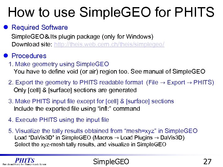How to use Simple. GEO for PHITS l Required Software Simple. GEO＆Its plugin package (only for Windows) Download site: http: //theis. web. cern. ch/theis/simplegeo/ l Procedures 1. Make geometry using Simple. GEO You have to define void (or air) region too. See manual of Simple. GEO 2. Export the geometry to PHITS readable format (File → Export → PHITS) Only [cell] & [surface] sections are generated 3. Make PHITS input file except for [cell] & [surface] sections Include the exported file using “infl: ” command 4. Execute PHITS using the input file 5. Visualize the tally results obtained from “mesh=xyz” in Simple. GEO Load “Da. Vis 3 D” in Simple. GEO (Macros → Load Plugins → Da. Vis 3 D) Select the xyz-mesh tally results, and visualize in Simple. GEO 27

Change Geometry in Simple. GEO doll. pht [Cell] c Body 00001 26 -1 -1 c Eyes 00002 11 -7. 87 -6 : -3 c Head 00003 6 -1. 9 -2 #2 c Void 00004 0 -4 +1 #2 #3 +7 +8 c Outervoid 00005 -1 -5 +4 c leg 1 00006 26 -1 -7 c leg 2 00007 26 -1 -8 [Surface] c Body 1 RCC 0. 00 10. 00 5. 00 c Headball 2 SPH 0. 00 15. 00 c Left. Eye 3 SPH -3. 00 4. 00 16. 00 1. 00 c Outer. Sphere 4 SPH 0. 00 100. 00 c Outmostsphere 5 SPH 0. 00 100. 00 c Right. Eye 6 SPH 3. 00 4. 00 16. 00 1. 00 c leg 1 7 RCC -2. 50 0. 00 -10. 00 10. 00 2. 00 c leg 2 8 RCC 2. 50 0. 00 -10. 00 10. 00 2. 00 Export to PHITS Simple. GEO 28

Visualize Tally Result in 3 D Simple. GEO. inp [ T - Deposit ] title = [t-deposit] in xyz mesh = xyz # mesh type is xyz scoring mesh x-type = 2 # x-mesh is linear given by xmin, xmax and nx xmin = -5. 000000 # minimum value of x-mesh points xmax = 5. 000000 # maximum value of x-mesh points nx = 20 # number of x-mesh points y-type = 2 # y-mesh is linear given by ymin, ymax and ny ymin = -5. 000000 # minimum value of y-mesh points ymax = 5. 000000 # maximum value of y-mesh points ny = 20 # number of y-mesh points z-type = 2 # z-mesh is linear given by zmin, zmax and nz zmin = -10. 000000 # minimum value of z-mesh points zmax = 20. 00000 # maximum value of z-mesh points nz = 40 # number of z-mesh points Execute Extend the tally region Simple. GEO 1. Select ‘Macros -> Load Plugins -> Da. Vis 3 D’ 2. Press ‘Da. Vis 3 D‘ button 3. Select ‘deposity-xy. out’ and press ‘Load data’ Simple. GEO 29

Contents • Recommendation Settings • Particle. Therapy • H 10 mupliplier • Utilities • Animation of Particle Trajectories • Simple. GEO • Summary and Homework Contents 30

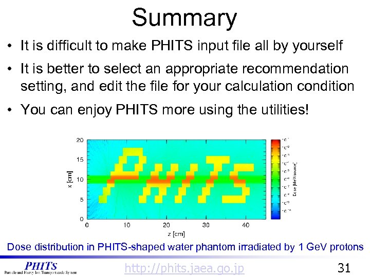Summary • It is difficult to make PHITS input file all by yourself • It is better to select an appropriate recommendation setting, and edit the file for your calculation condition • You can enjoy PHITS more using the utilities! Dose distribution in PHITS-shaped water phantom irradiated by 1 Ge. V protons http: //phits. jaea. go. jp 31

Homework 1. Calculate the depth-dose distributions for various radial distances inside cylindrical water phantom irradiated by 11 B 250 Me. V/u beam 2. Separate the depth-dose distributions into the contributions from neutron, proton, He, Li, Be, B 3. Divide the phantom into 2 layers, composed of water and Aluminum (2. 7 g/cm 3) respectively. 4. Obtain better statistic data by increasing the history number or by using the restart function Hints • • • Use 1 st [t-deposit] tally in “Particle. Therapy” in “recommendation” folder Increase the number of the radial bins in the [t-deposit] tally Comment out unnecessary tallies using “off” command for speed up Setup appropriate source particles and energy in [source] section Specify particle type in the [t-deposit] tally Add new material (Al), surface, and cells to set up geometry Summary 32

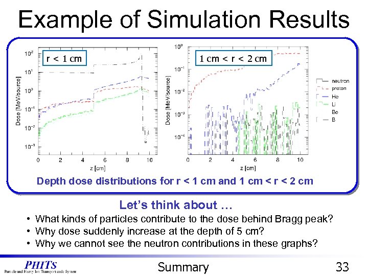Example of Simulation Results r < 1 cm < r < 2 cm Depth dose distributions for r < 1 cm and 1 cm < r < 2 cm Let’s think about … • What kinds of particles contribute to the dose behind Bragg peak? • Why dose suddenly increase at the depth of 5 cm? • Why we cannot see the neutron contributions in these graphs? Summary 33