4ebe87dcc0f661f45980918df501971d.ppt
- Количество слайдов: 158
Petri nets Classical Petri nets: The basic model 1
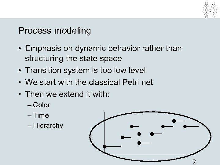
Process modeling • Emphasis on dynamic behavior rather than structuring the state space • Transition system is too low level • We start with the classical Petri net • Then we extend it with: – Color – Time – Hierarchy 2
Classical Petri net • Simple process model – Just three elements: places, transitions and arcs. – Graphical and mathematical description. – Formal semantics and allows for analysis. • History: – Carl Adam Petri (1962, Ph. D thesis) – In sixties and seventies focus mainly on theory. – Since eighties also focus on tools and applications (cf. CPN work by Kurt Jensen). – “Hidden” in many diagramming techniques and systems. 3
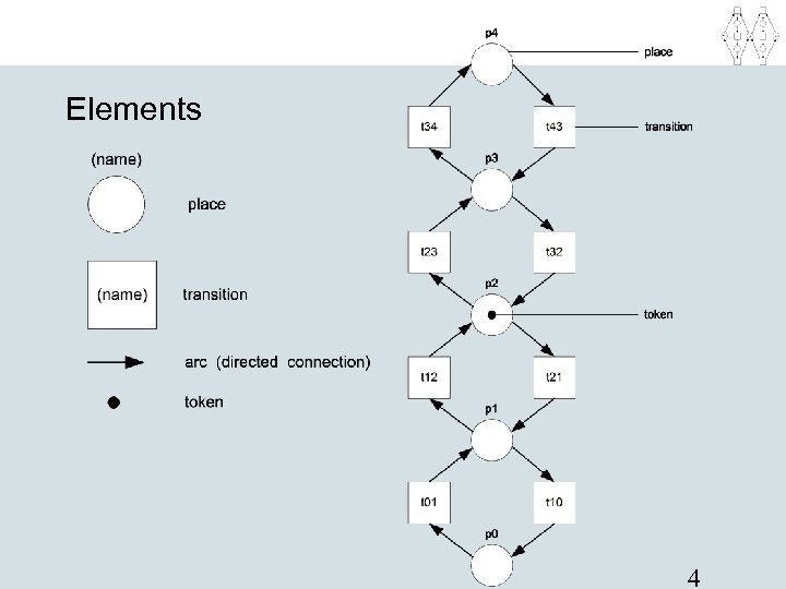
Elements 4
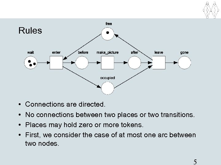
Rules • • Connections are directed. No connections between two places or two transitions. Places may hold zero or more tokens. First, we consider the case of at most one arc between two nodes. 5
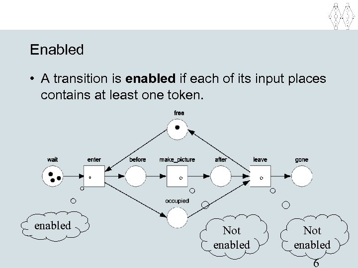
Enabled • A transition is enabled if each of its input places contains at least one token. enabled Not enabled 6
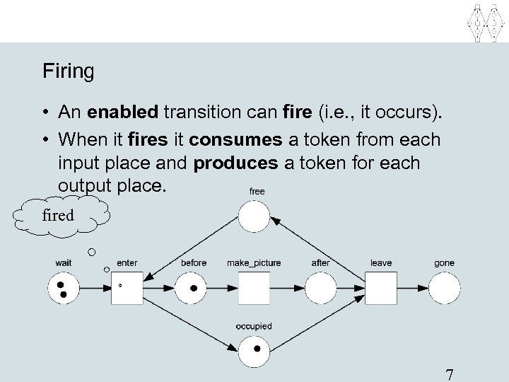
Firing • An enabled transition can fire (i. e. , it occurs). • When it fires it consumes a token from each input place and produces a token for each output place. fired 7
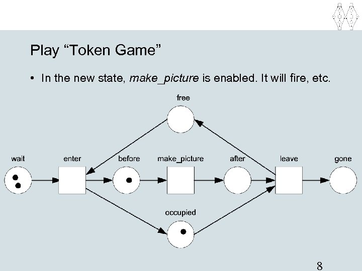
Play “Token Game” • In the new state, make_picture is enabled. It will fire, etc. 8
Remarks • Firing is atomic. • Multiple transitions may be enabled, but only one fires at a time, i. e. , we assume interleaving semantics (cf. diamond rule). • The number of tokens may vary if there are transitions for which the number of input places is not equal to the number of output places. • The network is static. • The state is represented by the distribution of tokens over places (also referred to as marking). 9
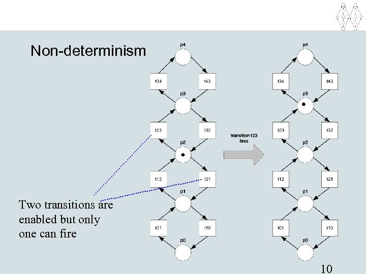
Non-determinism Two transitions are enabled but only one can fire 10
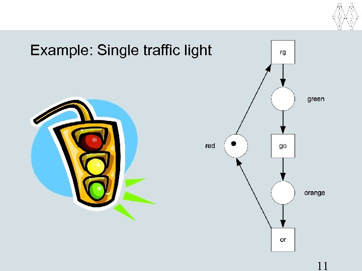
Example: Single traffic light 11
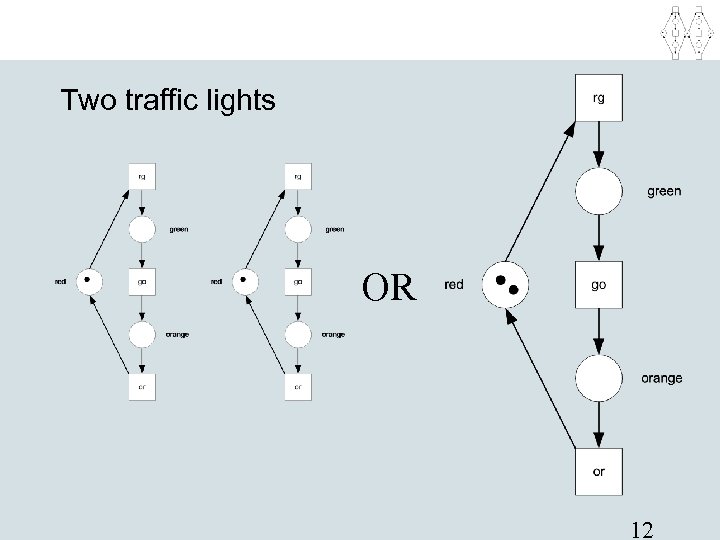
Two traffic lights OR 12
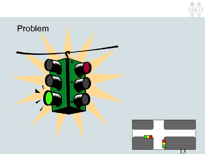
Problem 13
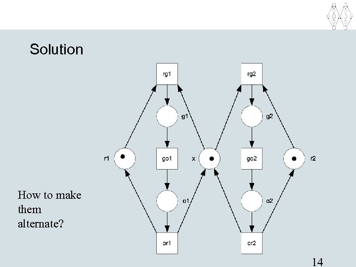
Solution How to make them alternate? 14
Playing the “Token Game” on the Internet • Applet to build your own Petri nets and execute them: http: //www. tm. tue. nl/it/staff/wvdaalst/Downloads/ pn_applet/pn_applet. html • FLASH animations: http: //www. tm. tue. nl/it/staff/wvdaalst/courses/pm /flash/ 15
Exercise: Train system (1) • Consider a circular railroad system with 4 (oneway) tracks (1, 2, 3, 4) and 2 trains (A, B). No two trains should be at the same track at the same time and we do not care about the identities of the two trains. 16
Exercise: Train system (2) • Consider a railroad system with 4 tracks (1, 2, 3, 4) and 2 trains (A, B). No two trains should be at the same track at the same time and we want to distinguish the two trains. 17
Exercise: Train system (3) • Consider a railroad system with 4 tracks (1, 2, 3, 4) and 2 trains (A, B). No two trains should be at the same track at the same time. Moreover the next track should also be free to allow for a safe distance. (We do not care about train identities. ) 18
Exercise: Train system (4) • Consider a railroad system with 4 tracks (1, 2, 3, 4) and 2 trains. Tracks are free, busy or claimed. Trains need to claim the next track before entering. 19

WARNING It is not sufficient to understand the (process) models. You have to be able to design them yourself ! 20
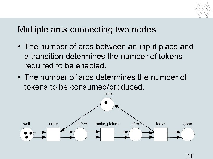
Multiple arcs connecting two nodes • The number of arcs between an input place and a transition determines the number of tokens required to be enabled. • The number of arcs determines the number of tokens to be consumed/produced. 21
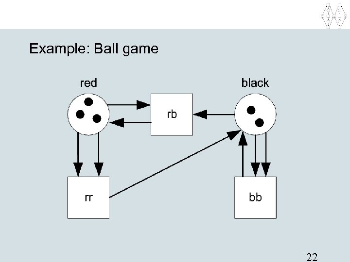
Example: Ball game 22
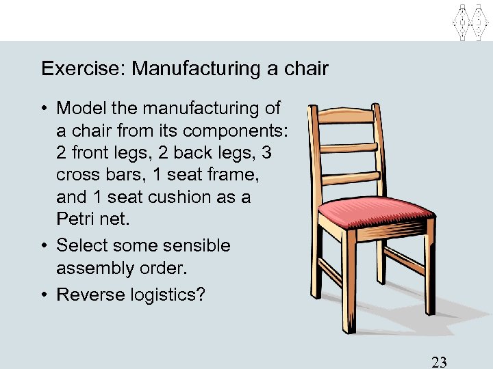
Exercise: Manufacturing a chair • Model the manufacturing of a chair from its components: 2 front legs, 2 back legs, 3 cross bars, 1 seat frame, and 1 seat cushion as a Petri net. • Select some sensible assembly order. • Reverse logistics? 23
Exercise: Burning alcohol. • Model C 2 H 5 OH + 3 * O 2 => 2 * CO 2 + 3 * H 2 O • Assume that there are two steps: first each molecule is disassembled into its atoms and then these atoms are assembled into other molecules. 24
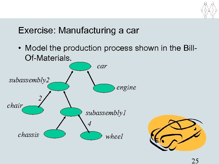
Exercise: Manufacturing a car • Model the production process shown in the Bill. Of-Materials. car subassembly 2 chair engine 2 chassis subassembly 1 4 wheel 25
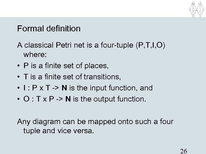
Formal definition A classical Petri net is a four-tuple (P, T, I, O) where: • P is a finite set of places, • T is a finite set of transitions, • I : P x T -> N is the input function, and • O : T x P -> N is the output function. Any diagram can be mapped onto such a four tuple and vice versa. 26
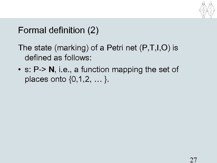
Formal definition (2) The state (marking) of a Petri net (P, T, I, O) is defined as follows: • s: P-> N, i. e. , a function mapping the set of places onto {0, 1, 2, … }. 27
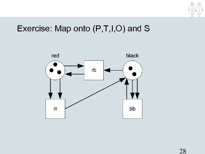
Exercise: Map onto (P, T, I, O) and S 28
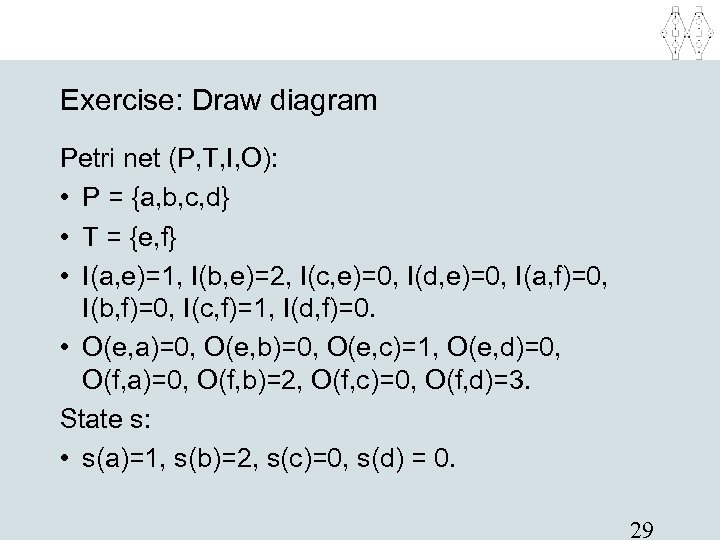
Exercise: Draw diagram Petri net (P, T, I, O): • P = {a, b, c, d} • T = {e, f} • I(a, e)=1, I(b, e)=2, I(c, e)=0, I(d, e)=0, I(a, f)=0, I(b, f)=0, I(c, f)=1, I(d, f)=0. • O(e, a)=0, O(e, b)=0, O(e, c)=1, O(e, d)=0, O(f, a)=0, O(f, b)=2, O(f, c)=0, O(f, d)=3. State s: • s(a)=1, s(b)=2, s(c)=0, s(d) = 0. 29
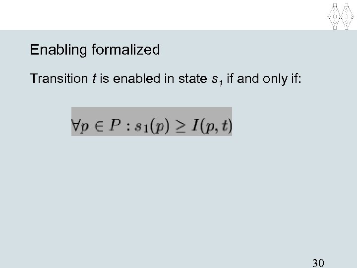
Enabling formalized Transition t is enabled in state s 1 if and only if: 30
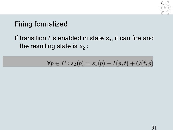
Firing formalized If transition t is enabled in state s 1, it can fire and the resulting state is s 2 : 31
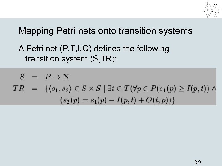
Mapping Petri nets onto transition systems A Petri net (P, T, I, O) defines the following transition system (S, TR): 32
Reachability graph • • The reachability graph of a Petri net is the part of the transition system reachable from the initial state in graph-like notation. The reachability graph can be calculated as follows: 1. Let X be the set containing just the initial state and let Y be the empty set. 2. Take an element x of X and add this to Y. Calculate all states reachable for x by firing some enabled transition. Each successor state that is not in Y is added to X. 3. If X is empty stop, otherwise goto 2. 33
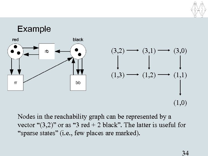
Example (3, 2) (3, 1) (3, 0) (1, 3) (1, 2) (1, 1) (1, 0) Nodes in the reachability graph can be represented by a vector “(3, 2)” or as “ 3 red + 2 black”. The latter is useful for “sparse states” (i. e. , few places are marked). 34
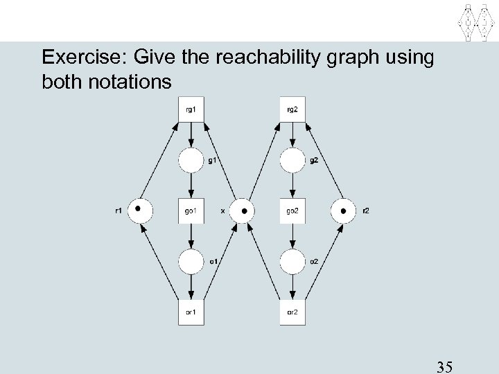
Exercise: Give the reachability graph using both notations 35
Different types of states • Initial state: Initial distribution of tokens. • Reachable state: Reachable from initial state. • Final state (also referred to as “dead states”): No transition is enabled. • Home state (also referred to as home marking): It is always possible to return (i. e. , it is reachable from any reachable state). How to recognize these states in the reachability graph? 36
Exercise: Producers and consumers • Model a process with one producer and one consumer, both are either busy or free and alternate between these two states. After every production cycle the producer puts a product in a buffer. The consumer consumes one product from this buffer per cycle. • Give the reachability graph and indicate the final states. • How to model 4 producers and 3 consumers connected through a single buffer? • How to limit the size of the buffer to 4? 37
Exercise: Two switches • Consider a room with two switches and one light. The light is on or off. The switches are in state up or down. At any time any of the switches can be used to turn the light on or off. • Model this as a Petri net. • Give the reachability graph. 38
Modeling • • Place: passive element Transition: active element Arc: causal relation Token: elements subject to change The state (space) of a process/system is modeled by places and tokens and state transitions are modeled by transitions (cf. transition systems). 39
Role of a token Tokens can play the following roles: • a physical object, for example a product, a part, a drug, a person; • an information object, for example a message, a signal, a report; • a collection of objects, for example a truck with products, a warehouse with parts, or an address file; • an indicator of a state, for example the indicator of the state in which a process is, or the state of an object; • an indicator of a condition: the presence of a token indicates whether a certain condition is fulfilled. 40
Role of a place • a type of communication medium, like a telephone line, a middleman, or a communication network; • a buffer: for example, a depot, a queue or a post bin; • a geographical location, like a place in a warehouse, office or hospital; • a possible state or state condition: for example, the floor where an elevator is, or the condition that a specialist is available. 41
Role of a transition • an event: for example, starting an operation, the death of a patient, a change seasons or the switching of a traffic light from red to green; • a transformation of an object, like adapting a product, updating a database, or updating a document; • a transport of an object: for example, transporting goods, or sending a file. 42
Typical network structures • • • Causality Parallelism (AND-split - AND-join) Choice (XOR-split – XOR-join) Iteration (XOR-join - XOR-split) Capacity constraints – Feedback loop – Mutual exclusion – Alternating 43
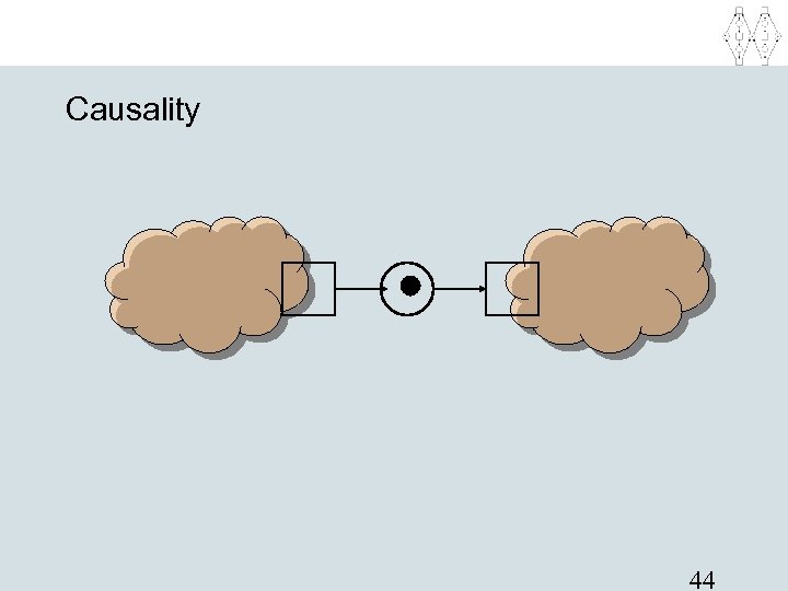
Causality 44
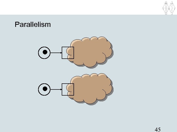
Parallelism 45
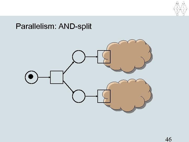
Parallelism: AND-split 46
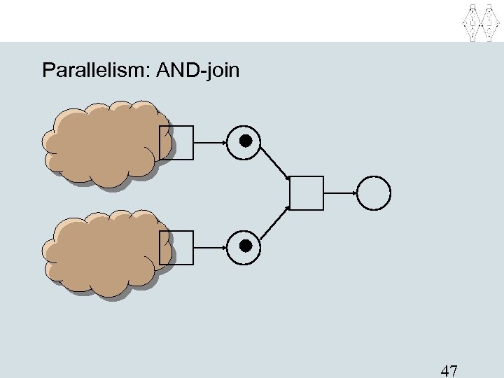
Parallelism: AND-join 47
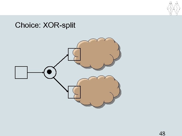
Choice: XOR-split 48
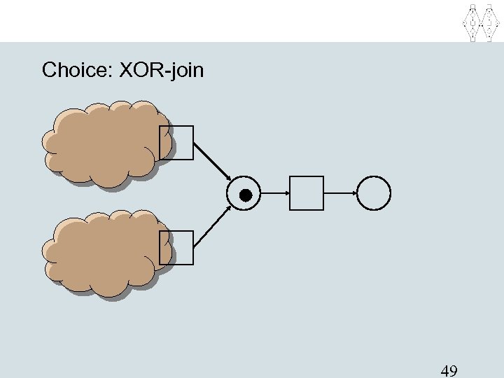
Choice: XOR-join 49
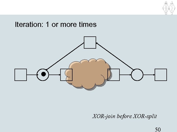
Iteration: 1 or more times XOR-join before XOR-split 50
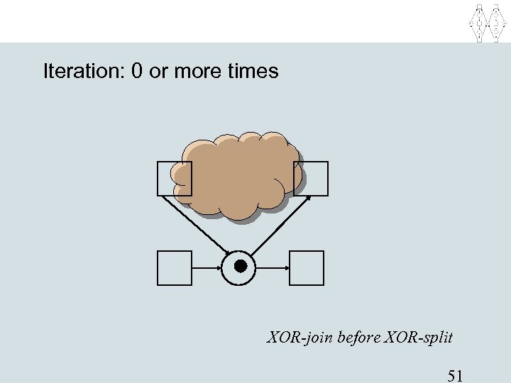
Iteration: 0 or more times XOR-join before XOR-split 51
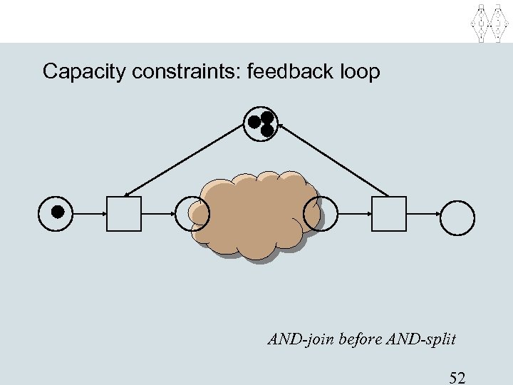
Capacity constraints: feedback loop AND-join before AND-split 52
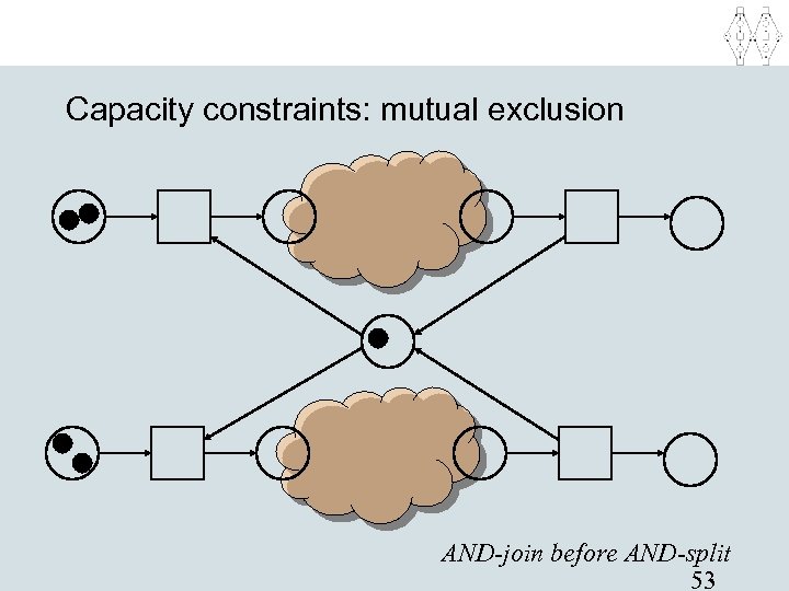
Capacity constraints: mutual exclusion AND-join before AND-split 53
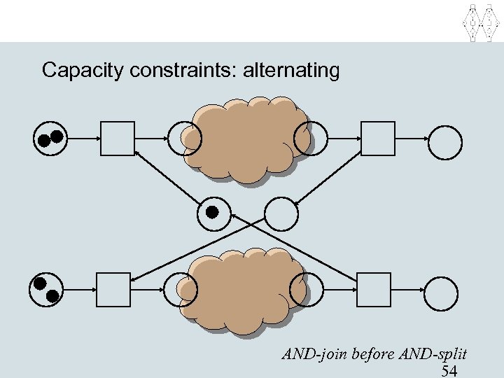
Capacity constraints: alternating AND-join before AND-split 54
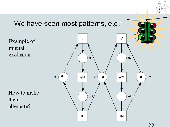
We have seen most patterns, e. g. : Example of mutual exclusion How to make them alternate? 55
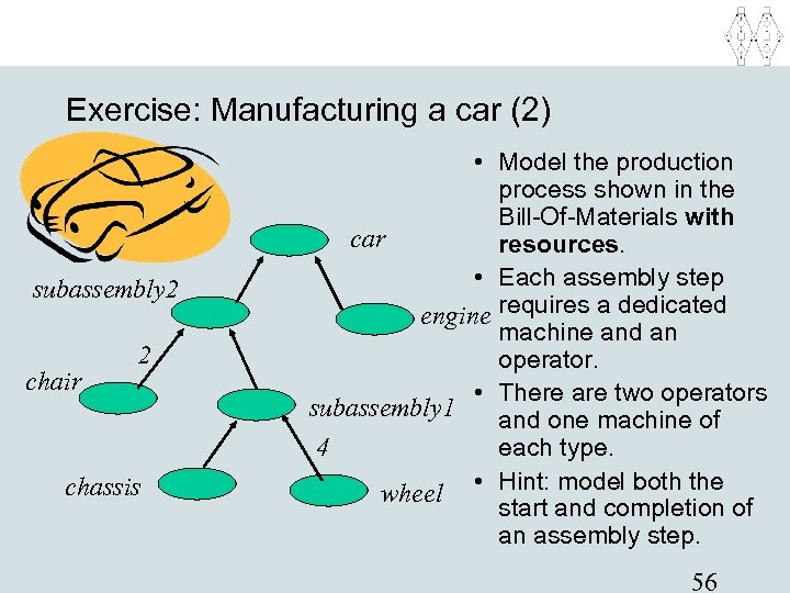
Exercise: Manufacturing a car (2) subassembly 2 chair 2 chassis • Model the production process shown in the Bill-Of-Materials with car resources. • Each assembly step engine requires a dedicated machine and an operator. • There are two operators subassembly 1 and one machine of each type. 4 wheel • Hint: model both the start and completion of an assembly step. 56
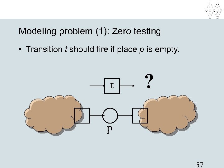
Modeling problem (1): Zero testing • Transition t should fire if place p is empty. t ? p 57
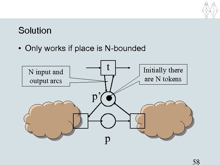
Solution • Only works if place is N-bounded t N input and output arcs Initially there are N tokens p’ p 58
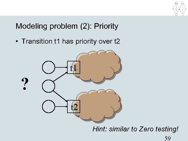
Modeling problem (2): Priority • Transition t 1 has priority over t 2 t 1 ? t 2 Hint: similar to Zero testing! 59
A bit of theory • Extensions have been proposed to tackle these problems, e. g. , inhibitor arcs. • These extensions extend the modeling power (Turing completeness*). • Without such an extension not Turing complete. • Still certain questions are difficult/expensive to answer or even undecidable (e. g. , equivalence of two nets). * Turing completeness corresponds to the ability to execute any computation. 60
Exercise: Witness statements • As part of the process of handling insurance claims there is the handling of witness statements. • There may be 0 -10 witnesses per claim. After an initialization step (one per claim), each of the witnesses is registered, contacted, and informed (i. e. , 0 -10 per claim in parallel). Only after all witness statements have been processed a report is made (one per claim). • Model this in terms of a Petri net. 61
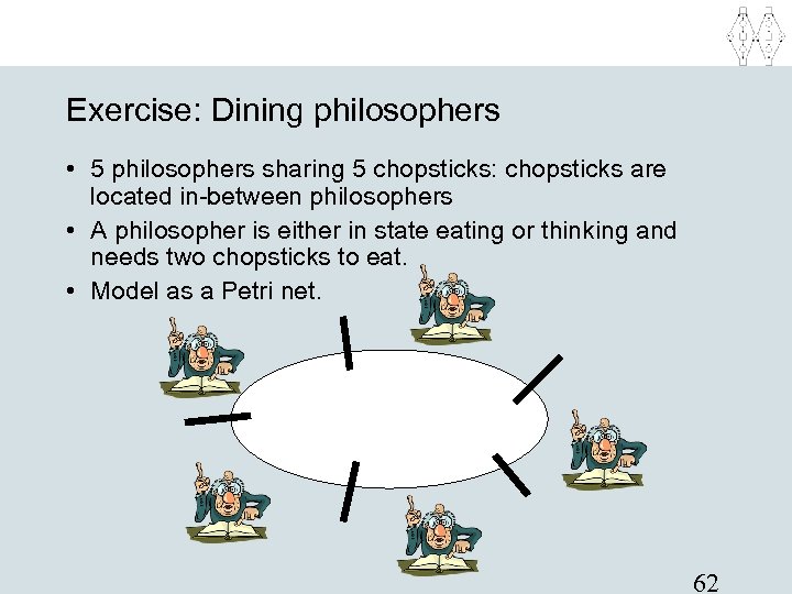
Exercise: Dining philosophers • 5 philosophers sharing 5 chopsticks: chopsticks are located in-between philosophers • A philosopher is either in state eating or thinking and needs two chopsticks to eat. • Model as a Petri net. 62

High level Petri nets Extending classical Petri nets with color, time and hierarchy (informal introduction) Prof. dr. ir. Wil van der Aalst Eindhoven University of Technology, Faculty of Technology Management, Department of Information and Technology, P. O. Box 513, NL-5600 MB, Eindhoven, The Netherlands. 63
Limitations of classical Petri nets • • Inability to test for zero tokens in a place. Models tend to become large. Models cannot reflect temporal aspects No support for structuring large models, cf. topdown and bottom-up design 64
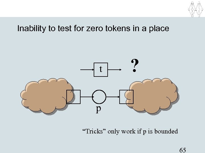
Inability to test for zero tokens in a place t ? p “Tricks” only work if p is bounded 65
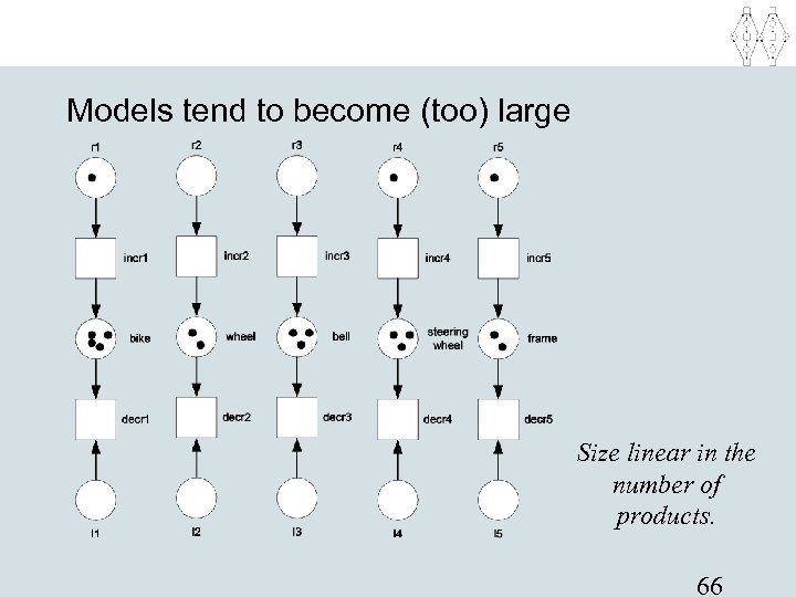
Models tend to become (too) large Size linear in the number of products. 66
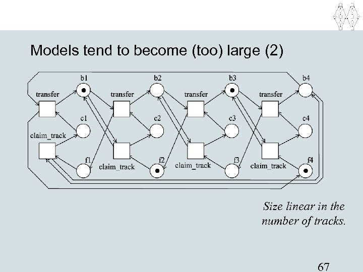
Models tend to become (too) large (2) Size linear in the number of tracks. 67
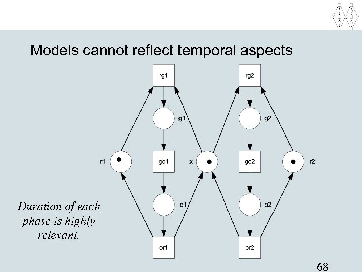
Models cannot reflect temporal aspects Duration of each phase is highly relevant. 68
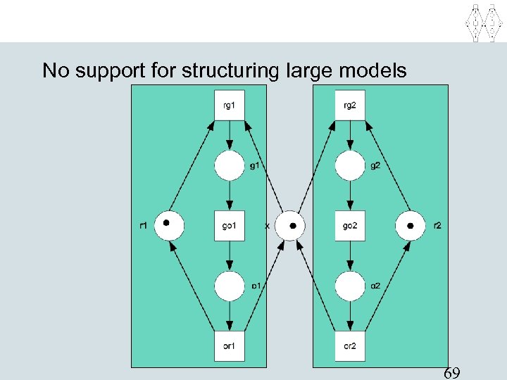
No support for structuring large models 69
High-level Petri nets • To tackle the problems identified. • Petri nets extended with: – Color (i. e. , data) – Time – Hierarchy • For the time being be do not choose a concrete language but focus on the main concepts. • Later we focus on a concrete language: CPN. • These concepts are supported by many variants of CPN including Ex. Spect, CPN AMI, etc. 70
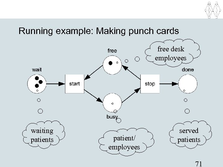
Running example: Making punch cards free desk employees waiting patients patient/ employees served patients 71
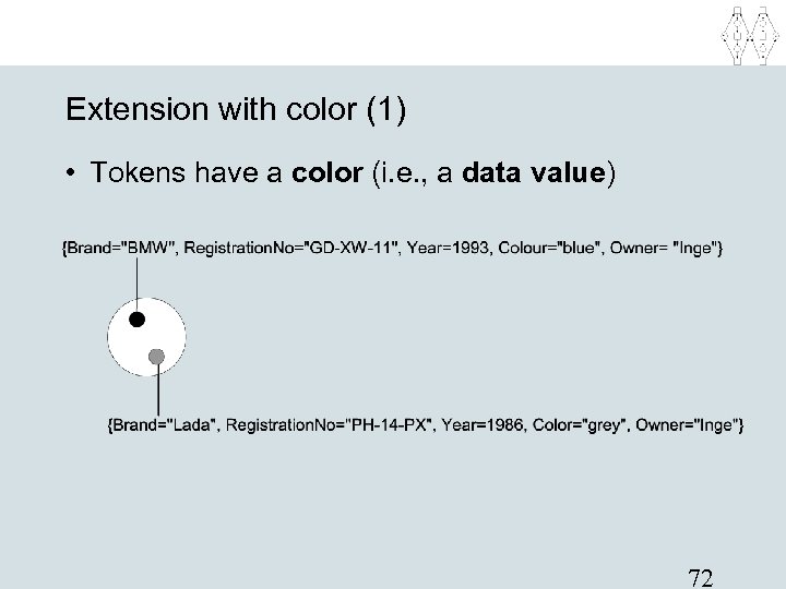
Extension with color (1) • Tokens have a color (i. e. , a data value) 72
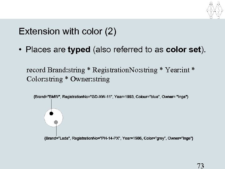
Extension with color (2) • Places are typed (also referred to as color set). record Brand: string * Registration. No: string * Year: int * Color: string * Owner: string 73
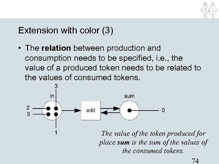
Extension with color (3) • The relation between production and consumption needs to be specified, i. e. , the value of a produced token needs to be related to the values of consumed tokens. The value of the token produced for place sum is the sum of the values of the consumed tokens. 74
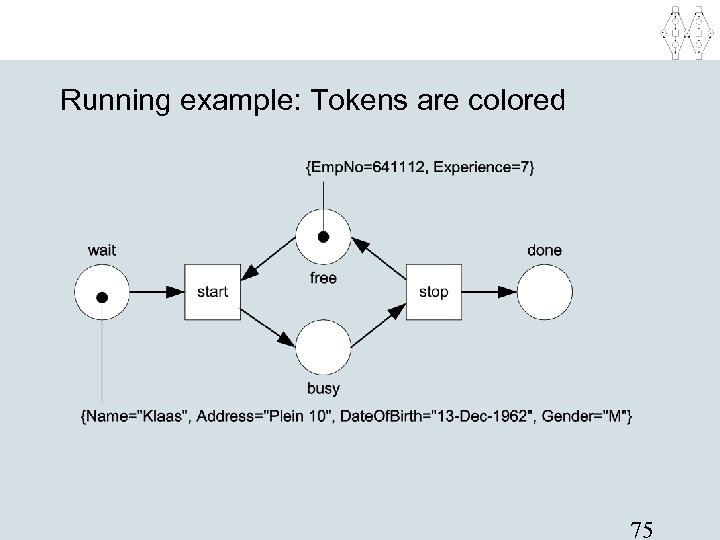
Running example: Tokens are colored 75
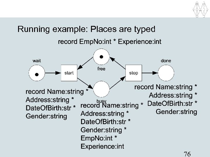
Running example: Places are typed 76
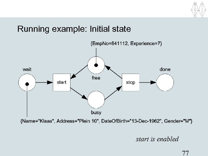
Running example: Initial state start is enabled 77
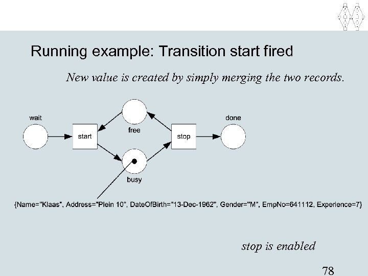
Running example: Transition start fired New value is created by simply merging the two records. stop is enabled 78
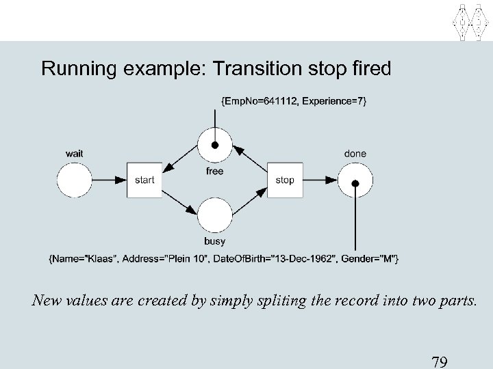
Running example: Transition stop fired New values are created by simply spliting the record into two parts. 79
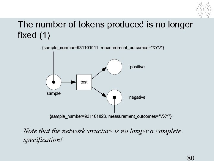
The number of tokens produced is no longer fixed (1) Note that the network structure is no longer a complete specification! 80
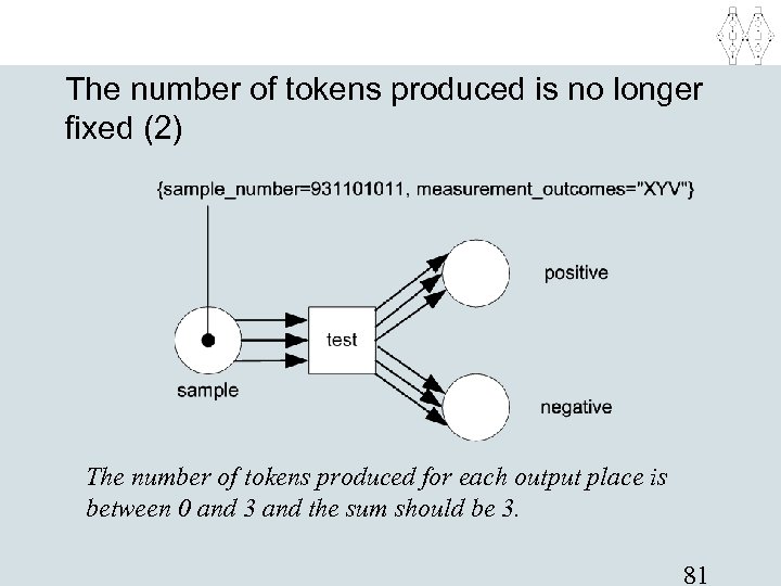
The number of tokens produced is no longer fixed (2) The number of tokens produced for each output place is between 0 and 3 and the sum should be 3. 81
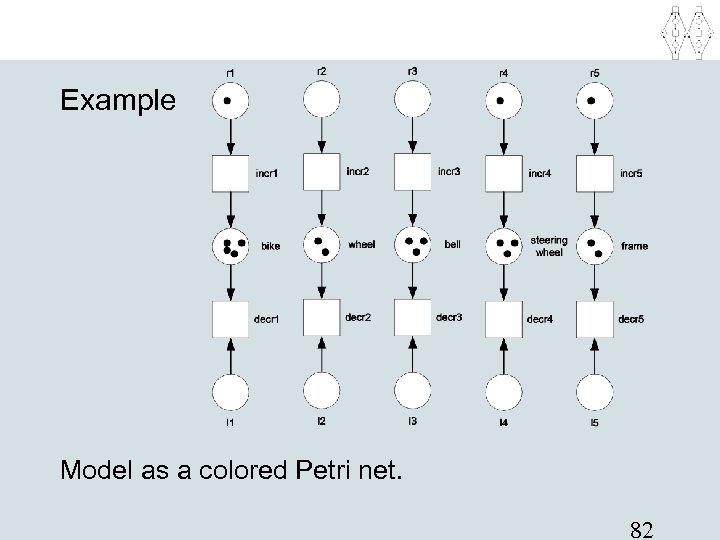
Example Model as a colored Petri net. 82
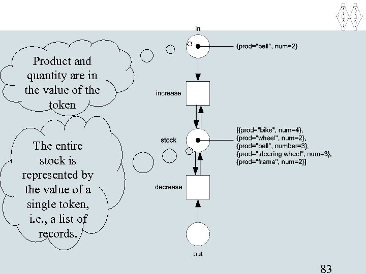
Product and quantity are in the value of the token The entire stock is represented by the value of a single token, i. e. , a list of records. 83
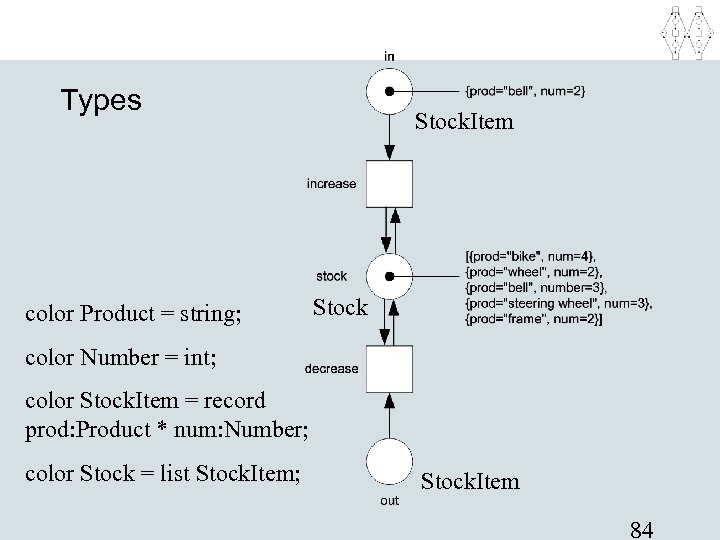
Types color Product = string; Stock. Item Stock color Number = int; color Stock. Item = record prod: Product * num: Number; color Stock = list Stock. Item; Stock. Item 84
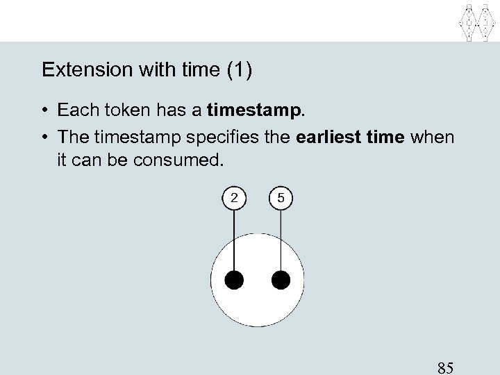
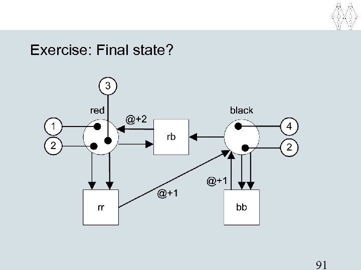
Extension with time (1) • Each token has a timestamp. • The timestamp specifies the earliest time when it can be consumed. 85
Extension with time (2) • The enabling time of a transition is the maximum of the tokens to be consumed. • If there are multiple tokens in a place, the earliest ones are consumed first. • A transition with the smallest firing time will fire first. • Transitions are eager, i. e. , they fire as soon as they can. • Produced token may have a delay. • The timestamp of a produced token is the firing time plus its delay. 86
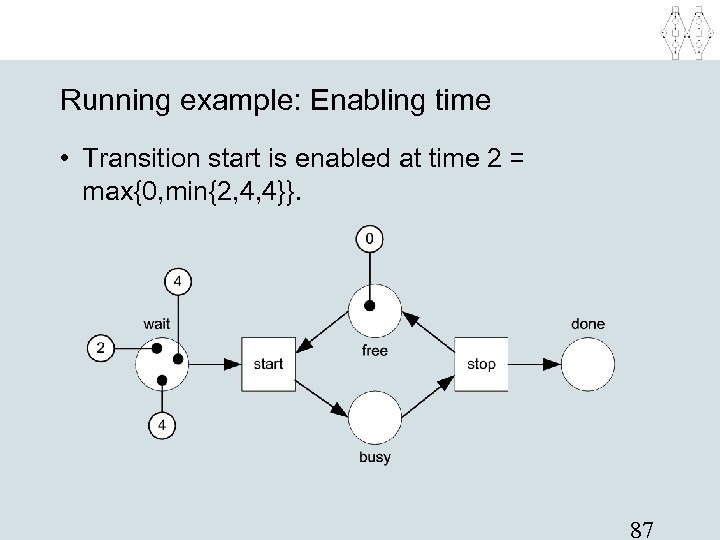
Running example: Enabling time • Transition start is enabled at time 2 = max{0, min{2, 4, 4}}. 87
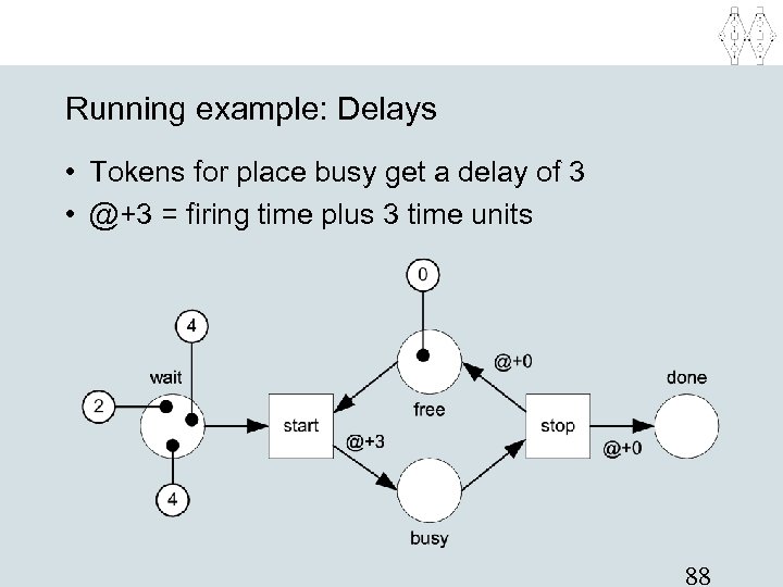
Running example: Delays • Tokens for place busy get a delay of 3 • @+3 = firing time plus 3 time units 88
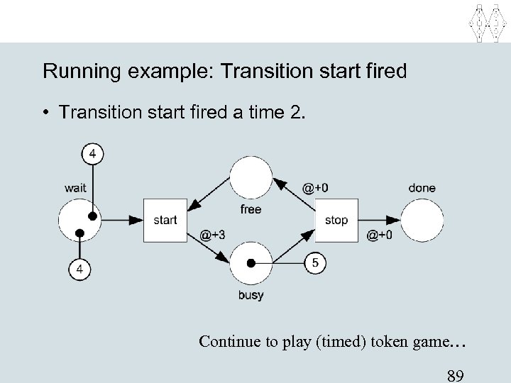
Running example: Transition start fired • Transition start fired a time 2. Continue to play (timed) token game… 89
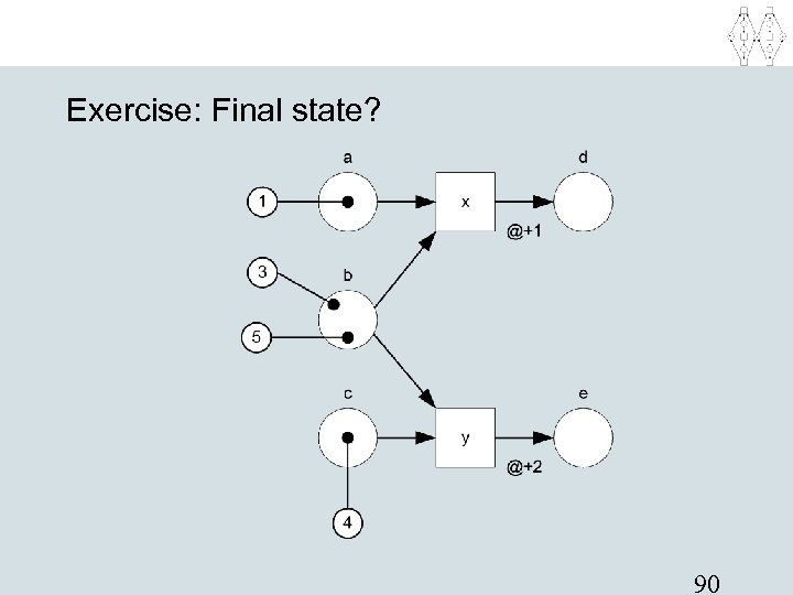
Exercise: Final state? 90
Exercise: Final state? 91
Extension with hierarchy • Timed and colored Petri nets result in more compact models. • However, for complex systems/processes the model does not fit on a single page. • Moreover, putting things at the same level does not reflect the structure of the process/system. • Many hierarchy concepts are possible. In this course we restrict ourselves to transition refinement. 92
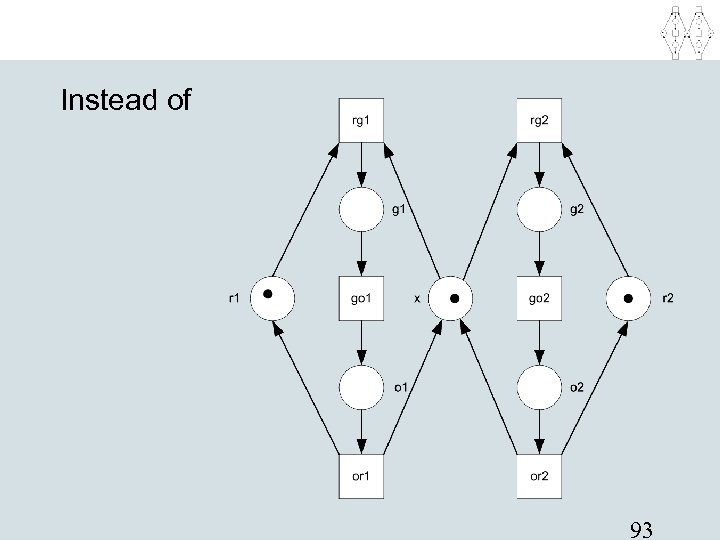
Instead of 93
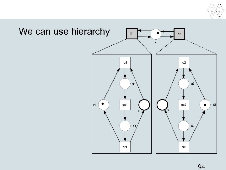
We can use hierarchy 94
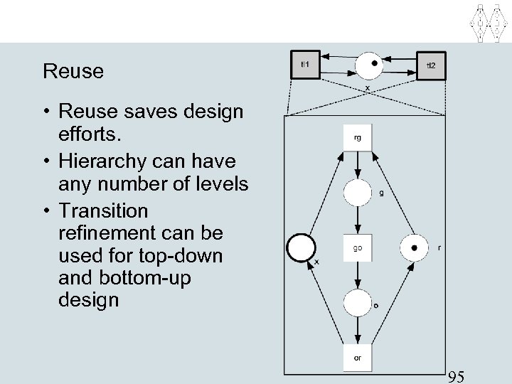
Reuse • Reuse saves design efforts. • Hierarchy can have any number of levels • Transition refinement can be used for top-down and bottom-up design 95
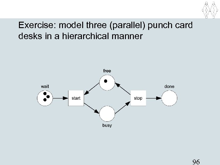
Exercise: model three (parallel) punch card desks in a hierarchical manner 96
Analysis of Process Models: Reachability graphs, invariants, and simulation Prof. dr. ir. Wil van der Aalst Eindhoven University of Technology, Faculty of Technology Management, Department of Information and Technology, P. O. Box 513, NL-5600 MB, Eindhoven, The Netherlands. 97
Questions raised when considering the handling of customer orders • • • How many orders arrive on average? How many orders can be handled? Do orders get lost? Do back orders always have priority? What is the utilization of office workers? If the desired product is no longer available, does the order get stuck? • Etc. 98
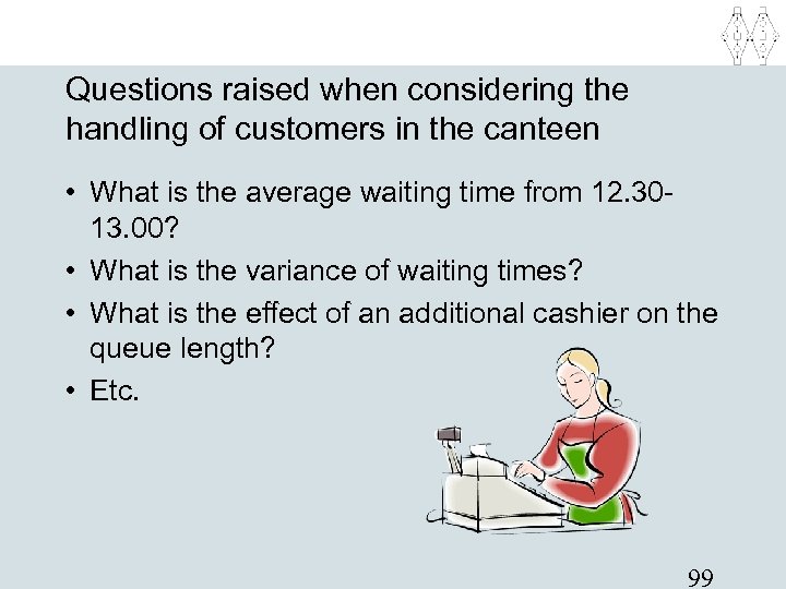
Questions raised when considering the handling of customers in the canteen • What is the average waiting time from 12. 3013. 00? • What is the variance of waiting times? • What is the effect of an additional cashier on the queue length? • Etc. 99
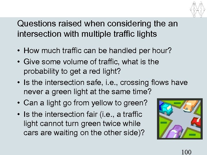
Questions raised when considering the an intersection with multiple traffic lights • How much traffic can be handled per hour? • Give some volume of traffic, what is the probability to get a red light? • Is the intersection safe, i. e. , crossing flows have never a green light at the same time? • Can a light go from yellow to green? • Is the intersection fair (i. e. , a traffic light cannot turn green twice while cars are waiting on the other side)? 100
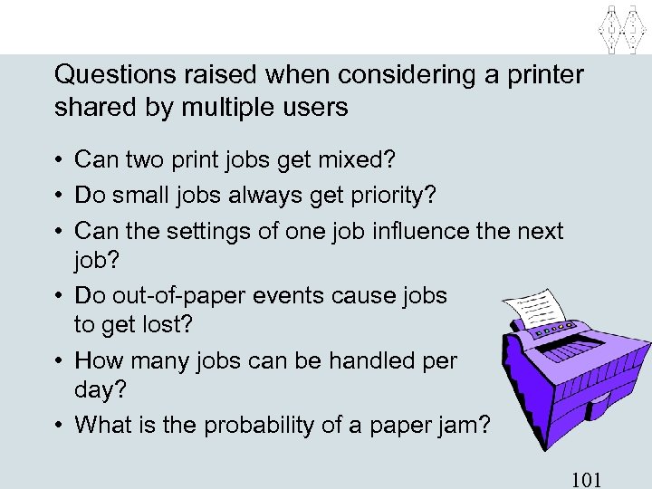
Questions raised when considering a printer shared by multiple users • Can two print jobs get mixed? • Do small jobs always get priority? • Can the settings of one job influence the next job? • Do out-of-paper events cause jobs to get lost? • How many jobs can be handled per day? • What is the probability of a paper jam? 101
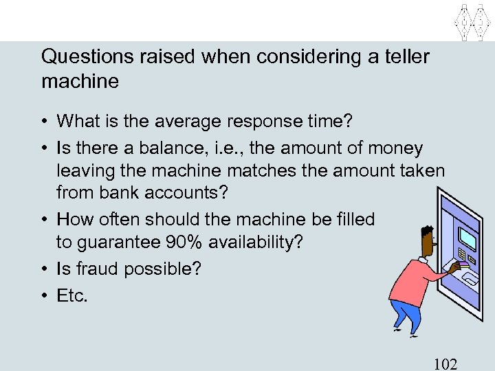
Questions raised when considering a teller machine • What is the average response time? • Is there a balance, i. e. , the amount of money leaving the machine matches the amount taken from bank accounts? • How often should the machine be filled to guarantee 90% availability? • Is fraud possible? • Etc. 102
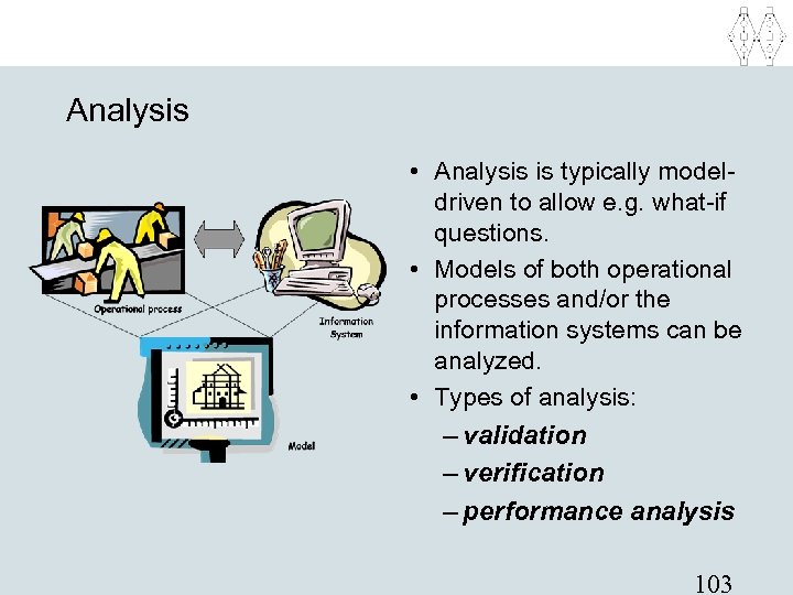
Analysis • Analysis is typically modeldriven to allow e. g. what-if questions. • Models of both operational processes and/or the information systems can be analyzed. • Types of analysis: – validation – verification – performance analysis 103
Three analysis techniques (Chapter 8) • Reachability graph • Place & transition invariants • Simulation • Each can be applied to both classical and high-level Petri nets. Nevertheless, for the first two we restrict ourselves to the classical Petri nets. • Use: – reachability graph (validation, verification) – invariants (validation, verification) – simulation (validation, performance analysis) 104
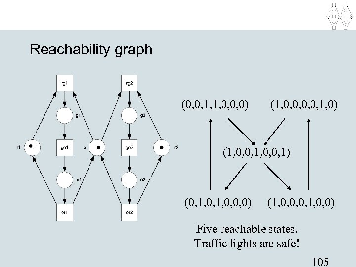
Reachability graph (0, 0, 1, 1, 0, 0, 0) (1, 0, 0, 1, 0) (1, 0, 0, 1) (0, 1, 0, 0, 0) (1, 0, 0, 0, 1, 0, 0) Five reachable states. Traffic lights are safe! 105
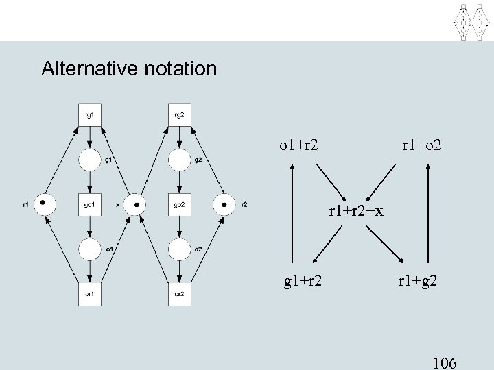
Alternative notation o 1+r 2 r 1+o 2 r 1+r 2+x g 1+r 2 r 1+g 2 106
Reachability graph (2) • Graph containing a node for each reachable state. • Constructed by starting in the initial state, calculate all directly reachable states, etc. • Expensive technique. • Only feasible if finitely many states (otherwise use coverability graph). • Difficult to generate diagnostic information. 107
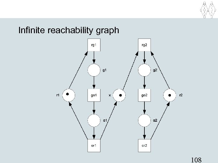
Infinite reachability graph 108
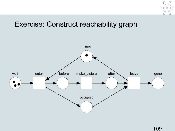
Exercise: Construct reachability graph 109
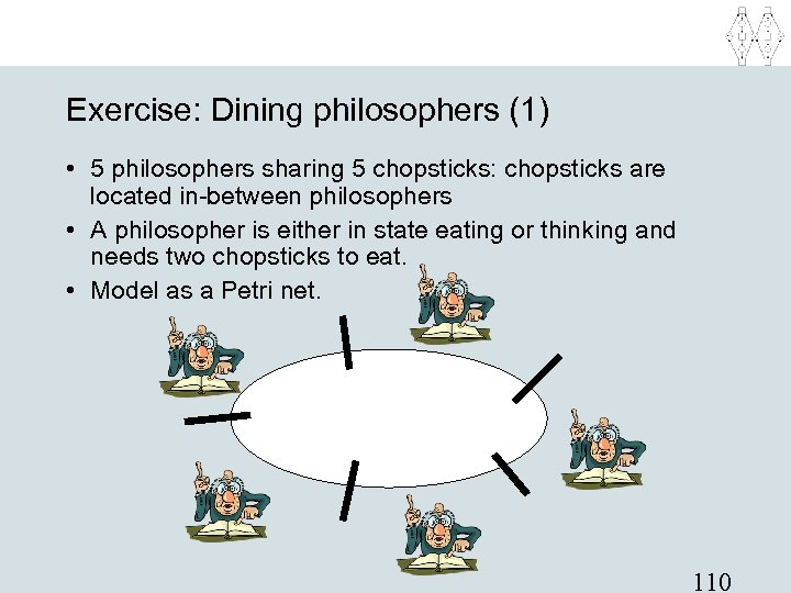
Exercise: Dining philosophers (1) • 5 philosophers sharing 5 chopsticks: chopsticks are located in-between philosophers • A philosopher is either in state eating or thinking and needs two chopsticks to eat. • Model as a Petri net. 110
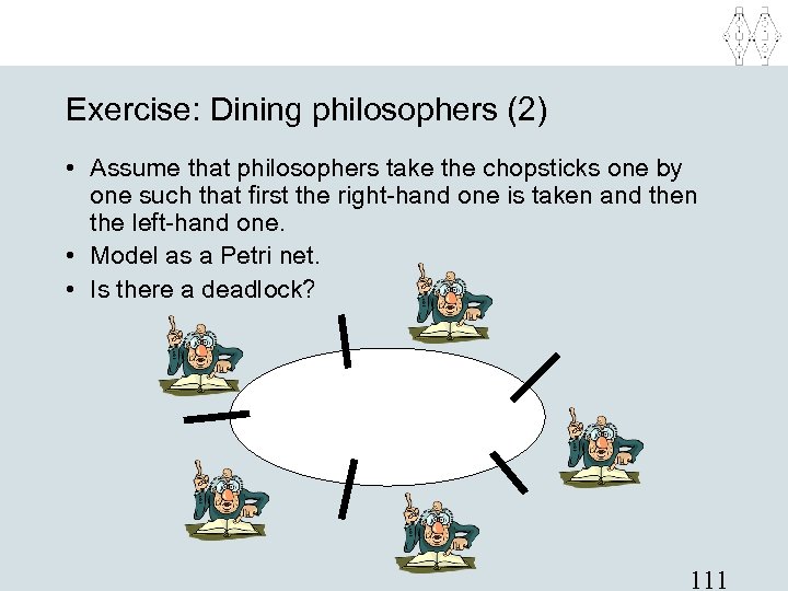
Exercise: Dining philosophers (2) • Assume that philosophers take the chopsticks one by one such that first the right-hand one is taken and then the left-hand one. • Model as a Petri net. • Is there a deadlock? 111
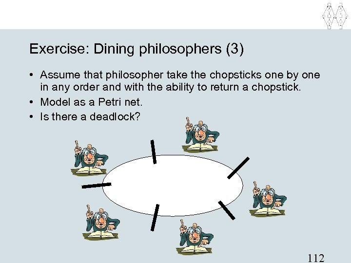
Exercise: Dining philosophers (3) • Assume that philosopher take the chopsticks one by one in any order and with the ability to return a chopstick. • Model as a Petri net. • Is there a deadlock? 112
Structural analysis techniques • To avoid state-explosion problem and bad diagnostics. • Properties independent of initial state. • We only consider place and transition invariants. • Invariants can be computed using linear algebraic techniques. 113
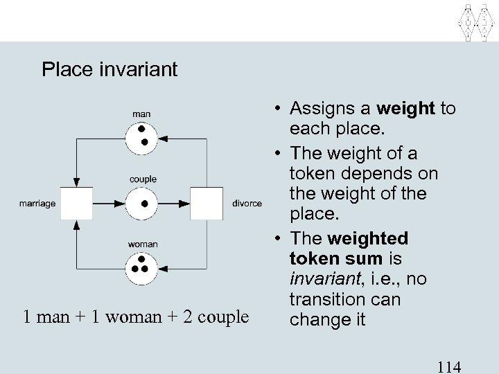
Place invariant 1 man + 1 woman + 2 couple • Assigns a weight to each place. • The weight of a token depends on the weight of the place. • The weighted token sum is invariant, i. e. , no transition can change it 114
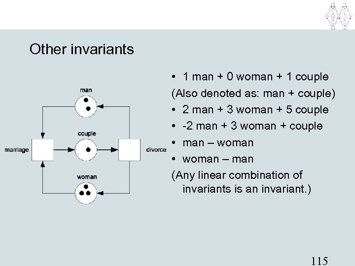
Other invariants • 1 man + 0 woman + 1 couple (Also denoted as: man + couple) • 2 man + 3 woman + 5 couple • -2 man + 3 woman + couple • man – woman • woman – man (Any linear combination of invariants is an invariant. ) 115
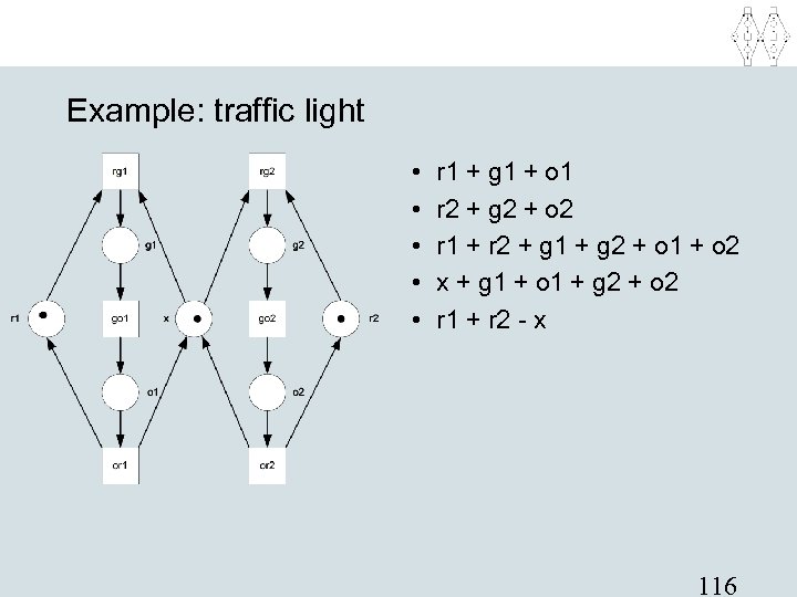
Example: traffic light • • • r 1 + g 1 + o 1 r 2 + g 2 + o 2 r 1 + r 2 + g 1 + g 2 + o 1 + o 2 x + g 1 + o 1 + g 2 + o 2 r 1 + r 2 - x 116
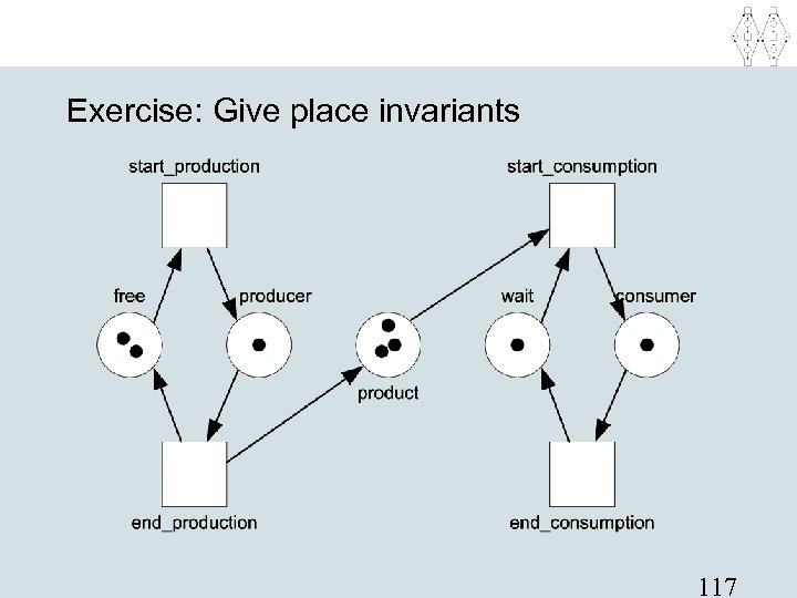
Exercise: Give place invariants 117
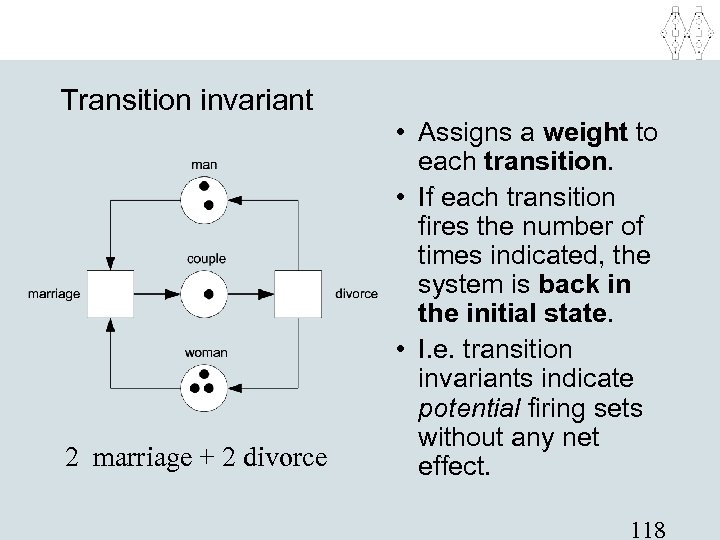
Transition invariant 2 marriage + 2 divorce • Assigns a weight to each transition. • If each transition fires the number of times indicated, the system is back in the initial state. • I. e. transition invariants indicate potential firing sets without any net effect. 118
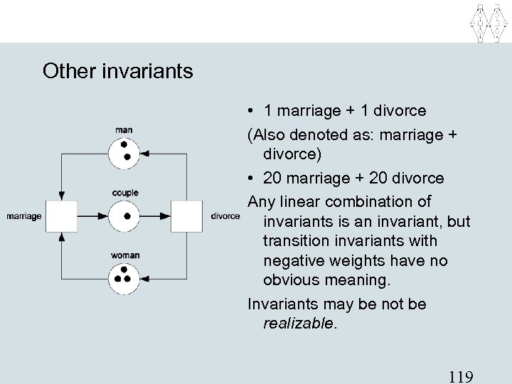
Other invariants • 1 marriage + 1 divorce (Also denoted as: marriage + divorce) • 20 marriage + 20 divorce Any linear combination of invariants is an invariant, but transition invariants with negative weights have no obvious meaning. Invariants may be not be realizable. 119
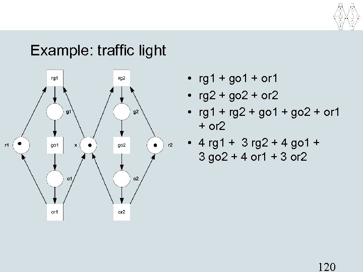
Example: traffic light • rg 1 + go 1 + or 1 • rg 2 + go 2 + or 2 • rg 1 + rg 2 + go 1 + go 2 + or 1 + or 2 • 4 rg 1 + 3 rg 2 + 4 go 1 + 3 go 2 + 4 or 1 + 3 or 2 120
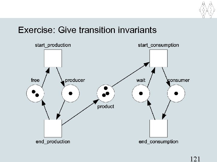
Exercise: Give transition invariants 121
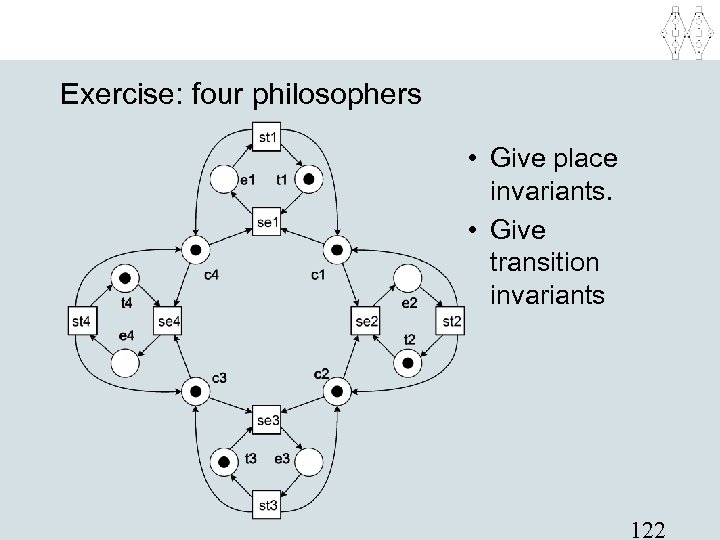
Exercise: four philosophers • Give place invariants. • Give transition invariants 122
Two ways of calculating invariants • "Intuitive way": Formulate the property that you think holds and verify it. • "Linear-algebraic way": Solve a system of linear equations. Humans tend to do it the intuitive way and computers do it the linear-algebraic way. 123
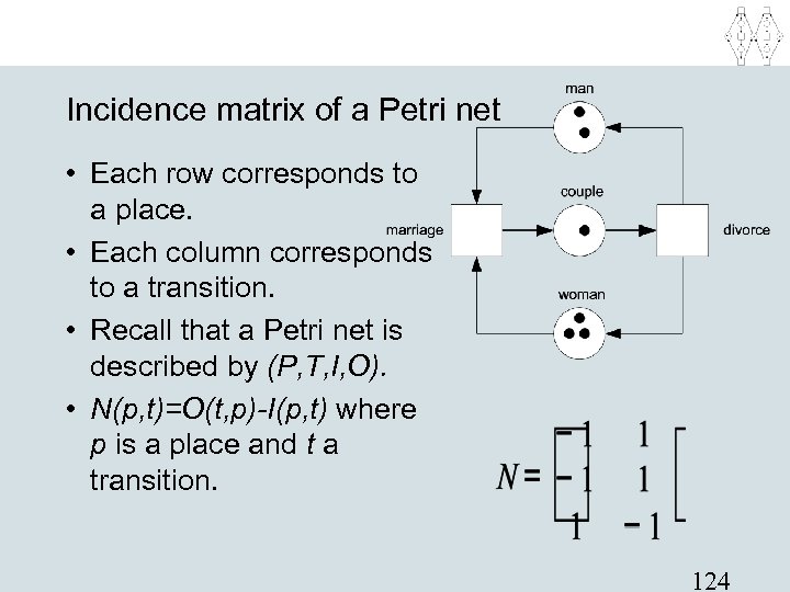
Incidence matrix of a Petri net • Each row corresponds to a place. • Each column corresponds to a transition. • Recall that a Petri net is described by (P, T, I, O). • N(p, t)=O(t, p)-I(p, t) where p is a place and t a transition. 124
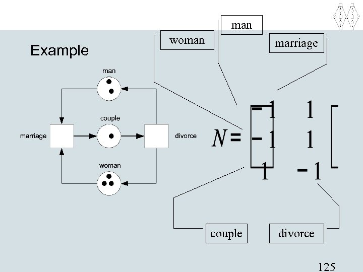
man Example woman marriage couple divorce 125
Place invariant • Let N be the incidence matrix of a net with n places and m transitions • Any solution of the equation X. N = 0 is a transition invariant – X is a row vector (i. e. , 1 x n matrix) – O is a row vector (i. e. , 1 x m matrix) • Note that (0, 0, . . . 0) is always a place invariant. • Basis can be calculated in polynomial time. 126
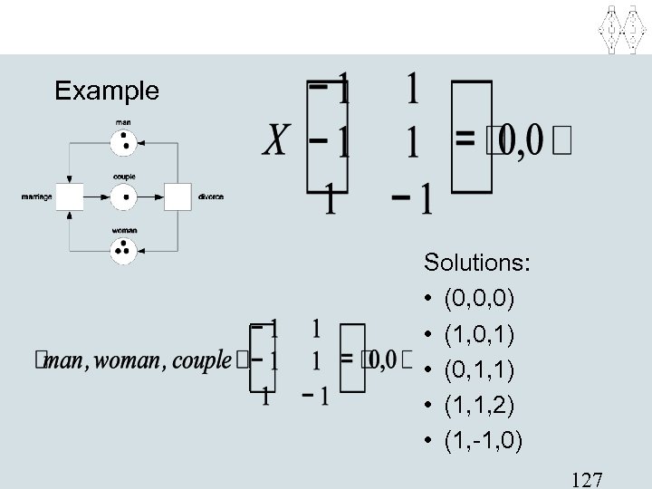
Example Solutions: • (0, 0, 0) • (1, 0, 1) • (0, 1, 1) • (1, 1, 2) • (1, -1, 0) 127
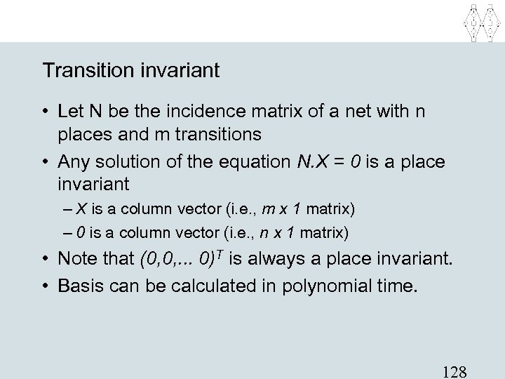
Transition invariant • Let N be the incidence matrix of a net with n places and m transitions • Any solution of the equation N. X = 0 is a place invariant – X is a column vector (i. e. , m x 1 matrix) – 0 is a column vector (i. e. , n x 1 matrix) • Note that (0, 0, . . . 0)T is always a place invariant. • Basis can be calculated in polynomial time. 128
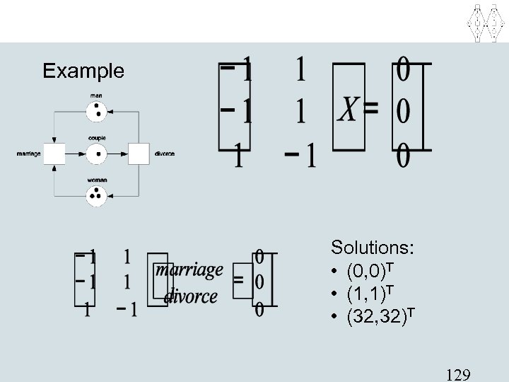
Example Solutions: • (0, 0)T • (1, 1)T • (32, 32)T 129
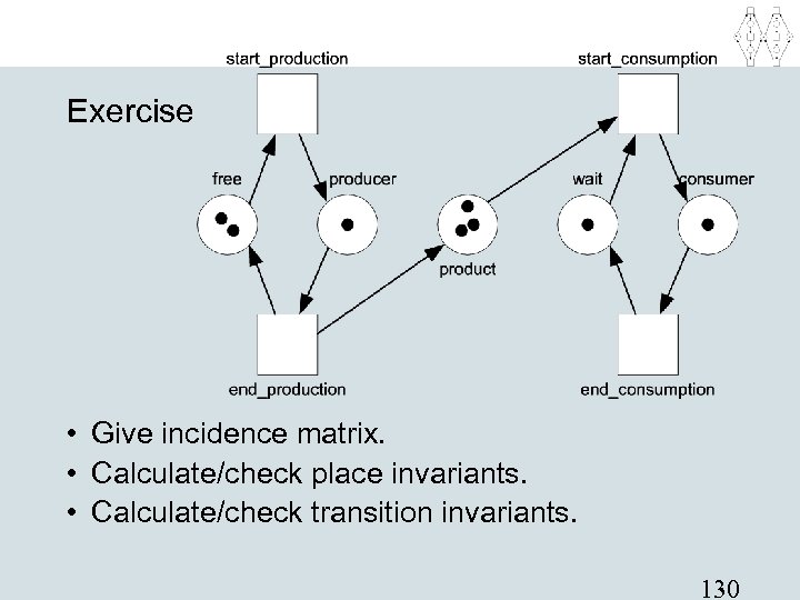
Exercise • Give incidence matrix. • Calculate/check place invariants. • Calculate/check transition invariants. 130
Simulation • Most widely used analysis technique. • From a technical point of view just a "walk" in the reachability graph. • By making many "walks" (in case of transient behavior) or a very "long walk" (in case of steady-state) behavior, it is possible to make reliable statements about properties/ performance indicators. • Used for validation and performance analysis. • Cannot be used to prove correctness! 131
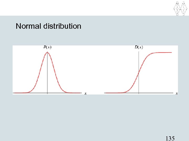
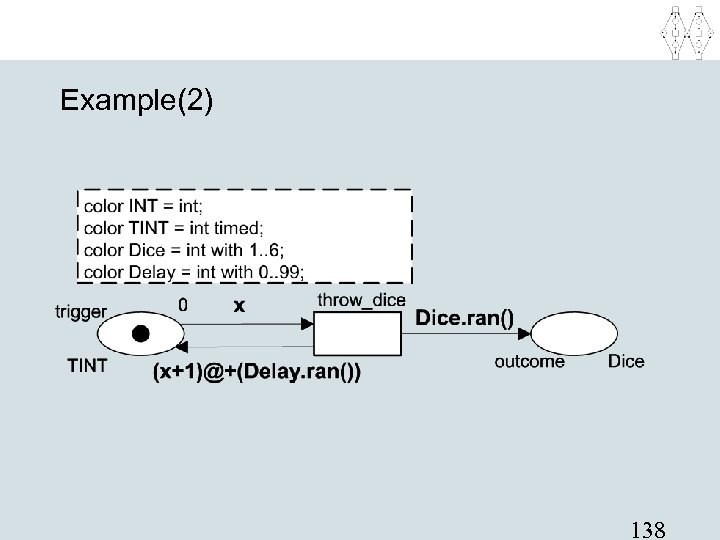
Stochastic process • Simulation of a deterministic system is not very interesting. • Simulation of an untimed system is not interesting. • In a timed and non-deterministic system, durations and probabilities are described by some probability distribution. • In other words, we simulate a stochastic process! • CPN allows for the use of distributions using some internal random generator. 132
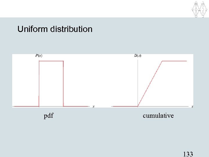
Uniform distribution pdf cumulative 133
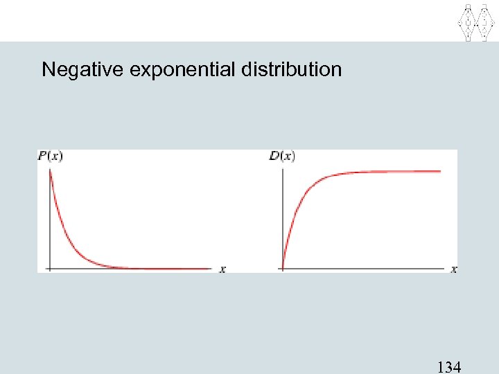
Negative exponential distribution 134
Normal distribution 135
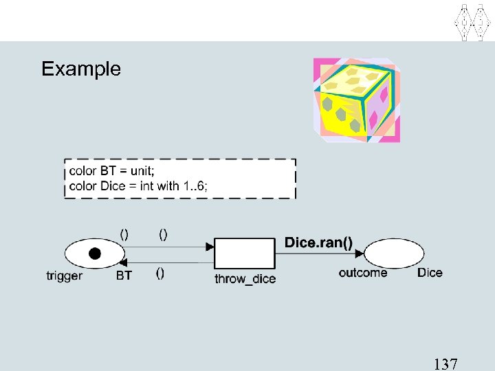
Distributions in CPN Tools Assume some library with functions: • uniform(x, y) • nexp(x) • erlang(n, x) • Etc. A nice function is also C. ran() which returns a randomly selected element of finite color set C, e. g. , color C = int with 1. . 5; fun select 1 to 5() = C. ran() returns a number between 1 and 5 136
Example 137
Example(2) 138
Subruns and confidence intervals • A single run does not provide information about reliability of results. • Therefore, multiple runs or one run cut into parts: subruns. • If the subruns are assumed to be mutually independent, one can calculate a confidence interval, e. g. , the flow time is with 95% confidence within the interval 5. 5+/-0. 5 (i. e. [5, 6]). 139
Example of a simulation model • Gas station with one pump and space for 4 cars (3 waiting and 1 being served). • Service time: uniform distribution between 2 and 5 minutes. • Poisson arrival process with mean time between arrivals of 4 minutes. • If there are more than 3 cars waiting, the "sale" is lost. • Questions: flow time, waiting time, utilization, lost sales, etc. 140
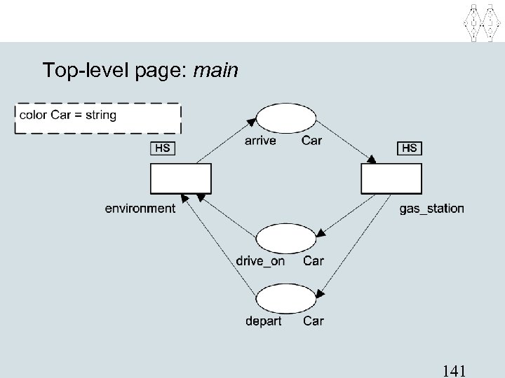
Top-level page: main 141
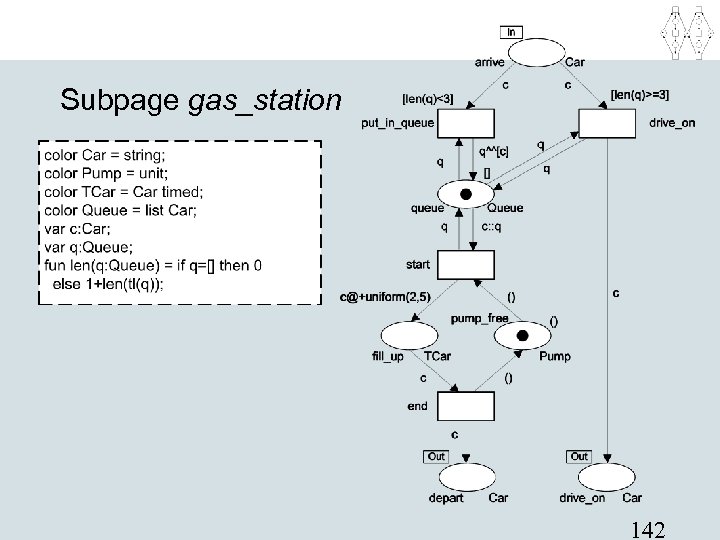
Subpage gas_station 142
Assuming pages for the environment and measurements the last two pages allow for. . . • Calculation of flow time (average, variance, maximum, minimum, service level, etc. ). • Calculation of waiting times (average, variance, maximum, minimum, service level, etc. ). • Calculation of lost sales (average). • Probability of no space left. • Probability of no cars waiting. For each of these metrics, it is possible to formulate a confidence interval given sufficient observations. 143
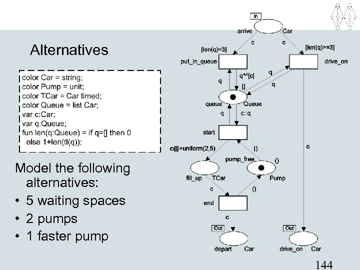
Alternatives Model the following alternatives: • 5 waiting spaces • 2 pumps • 1 faster pump 144
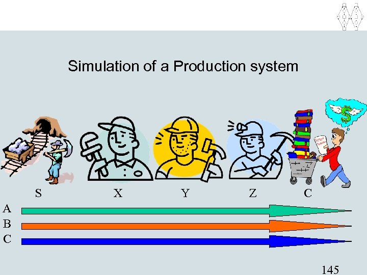
Simulation of a Production system S X Y Z C A B C 145
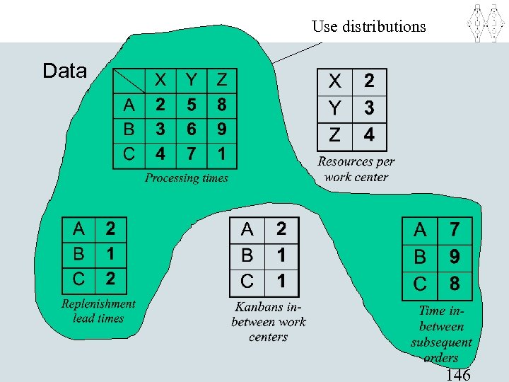
Use distributions Data 146
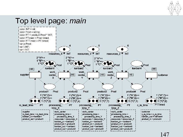
Top level page: main 147
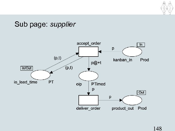
Sub page: supplier 148
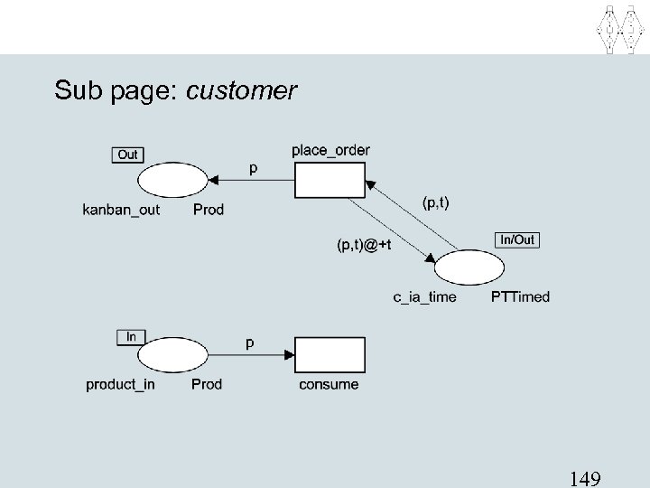
Sub page: customer 149
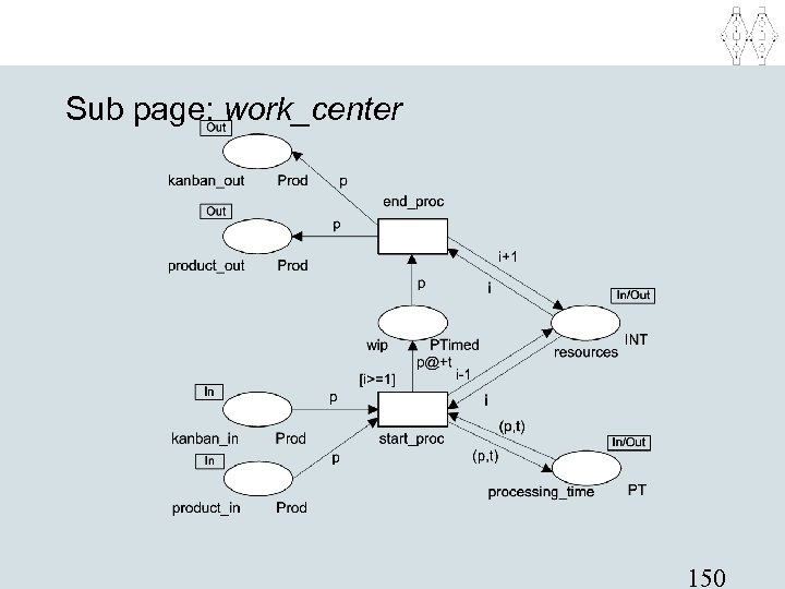
Sub page: work_center 150
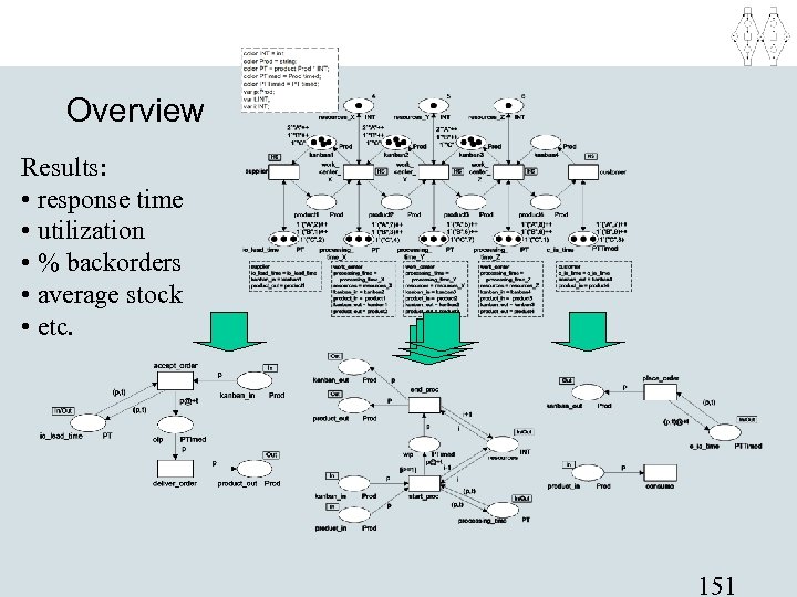
Overview Results: • response time • utilization • % backorders • average stock • etc. 151
Classical versus high-level Petri nets • • Simulation clearly works for all types of nets. Hierarchy is never a problem. Time allows for new types of analysis. Reachability graphs and invariants can also be extended to high-level nets. – More complex (both technique and computation) • Sometimes abstraction from color is possible to derive invariants (consider previous example). 152
Exercise: Five Chinese philosophers • Recall hierarchical CPN model of five Chinese philosophers alternating between states thinking and eating. – Give place invariants – Give transition invariants • Change the model such that philosophers can take one chopstick at a time but avoid deadlocks and a fixed ordering of philosophers. – Give place invariants – Give transition invariants 153
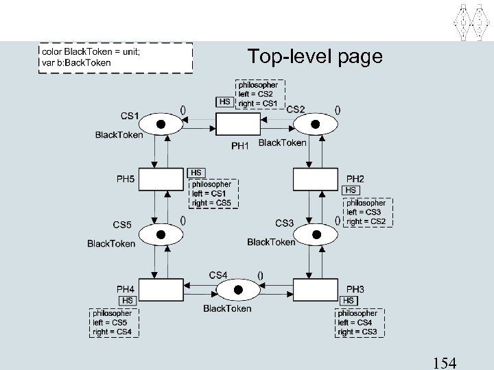
Top-level page 154
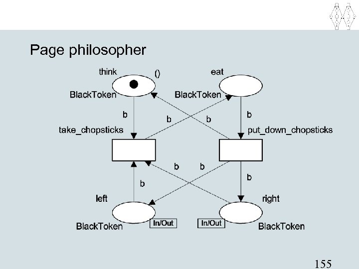
Page philosopher 155
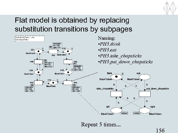
Flat model is obtained by replacing substitution transitions by subpages Naming: • PH 3. think • PH 3. eat • PH 3. take_chopsticks • PH 3. put_down_chopsticks Repeat 5 times. . . 156
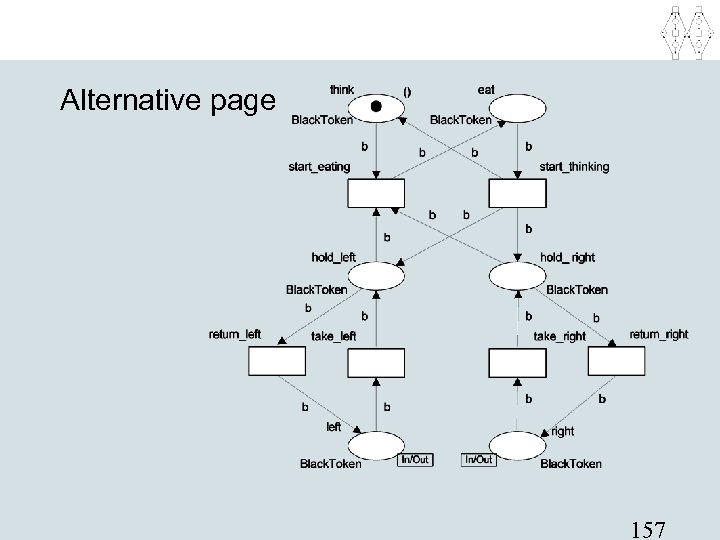
Alternative page 157
You should be able to. . . • Construct a reachability graph for a classical Petri net. • Give meaningful place and transition invariants for a classical Petri net. • Construct a reachability graph and give meaningful place and transition invariants for a hierarchical CPN after abstracting from data and time and removing hierarchy. • Build a simple simulation model using CPN. • Motivate the use of each of the analysis techniques. 158
4ebe87dcc0f661f45980918df501971d.ppt