Perfect Competition Copyright 2006 Pearson Education Canada

Perfect Competition Copyright © 2006 Pearson Education Canada 12 CHAPTER

Sweet Competition Maple syrup is produced by 12, 000 farms in Canada and the United States in a highly competitive market. We study such a market in this chapter. We explain the changes in price and output as the firms in perfect competition respond to changes in demand technological change. Copyright © 2006 Pearson Education Canada

Competition Perfect competition is an industry in which § Many firms sell identical products to many buyers. § There are no restrictions to entry into the industry. § Established firms have no advantages over new ones. § Sellers and buyers are well informed about prices. Copyright © 2006 Pearson Education Canada

Competition How Perfect Competition Arises Perfect competition arises § When firm’s minimum efficient scale is small relative to market demand so there is room for many firms in the industry. § And when each firm is perceived to produce a good or service that has no unique characteristics, so consumers don’t care which firm they buy from. Copyright © 2006 Pearson Education Canada

Competition Price Takers In perfect competition, each firm is a price taker. A price taker is a firm that cannot influence the price of a good or service. No single firm can influence the price—it must “take” the equilibrium market price. Each firm’s output is a perfect substitute for the output of the other firms, so the demand for each firm’s output is perfectly elastic. Copyright © 2006 Pearson Education Canada

Competition Economic Profit and Revenue The goal of each firm is to maximize economic profit, which equals total revenue minus total cost. Total cost is the opportunity cost of production, which includes normal profit. A firm’s total revenue equals price, P, multiplied by quantity sold, Q, or P Q. A firm’s marginal revenue is the change in total revenue that results from a one-unit increase in the quantity sold. Copyright © 2006 Pearson Education Canada

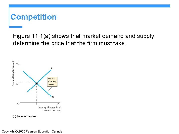Competition Figure 11. 1(a) shows that market demand supply determine the price that the firm must take. Copyright © 2006 Pearson Education Canada

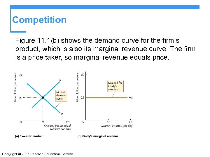Competition Figure 11. 1(b) shows the demand curve for the firm’s product, which is also its marginal revenue curve. The firm is a price taker, so marginal revenue equals price. Copyright © 2006 Pearson Education Canada

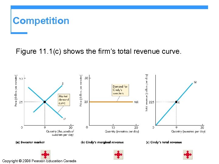Competition Figure 11. 1(c) shows the firm’s total revenue curve. Copyright © 2006 Pearson Education Canada

The Firm’s Decisions in Perfect Competition A perfectly competitive firm faces two constraints: 1. A market constraint summarized by the market price and the firm’s revenue curves 2. A technology constraint summarized by firm’s product curves and cost curves (like those in Chapter 10) Copyright © 2006 Pearson Education Canada

The Firm’s Decisions in Perfect Competition The competitive firm makes two decisions in the short run: 1. Whether to produce or to shut down. 2. If the decision is to produce, what quantity to produce. A firm’s long-run decisions are 1. Whether to increase or decrease its plant size. 2. Whether to stay in the industry or leave it. Copyright © 2006 Pearson Education Canada

The Firm’s Decisions in Perfect Competition Profit-Maximizing Output A perfectly competitive firm chooses the output that maximizes its economic profit. One way to find the profit-maximizing output is to look at the firm’s the total revenue and total cost curves. Figure 11. 2 on the next slide looks at these curves along with the firm’s total profit curve. Copyright © 2006 Pearson Education Canada

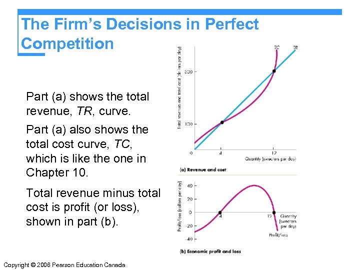The Firm’s Decisions in Perfect Competition Part (a) shows the total revenue, TR, curve. Part (a) also shows the total cost curve, TC, which is like the one in Chapter 10. Total revenue minus total cost is profit (or loss), shown in part (b). Copyright © 2006 Pearson Education Canada

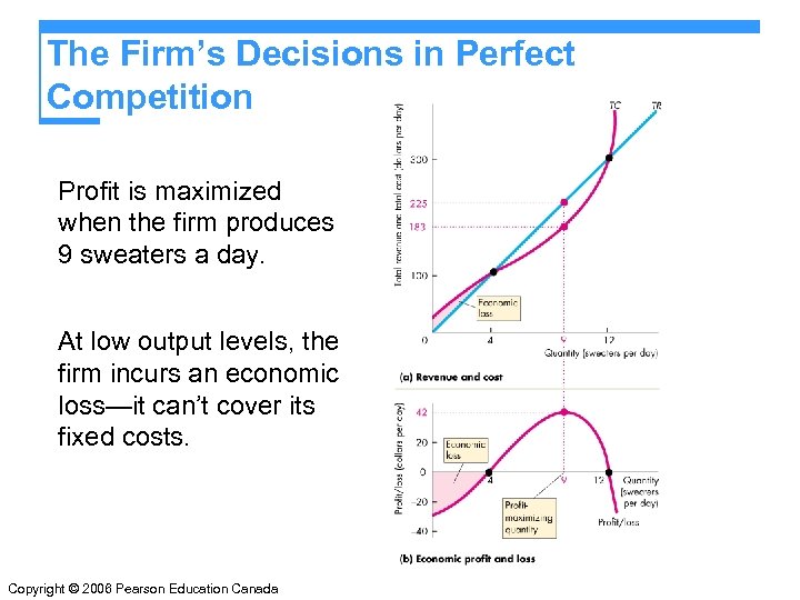The Firm’s Decisions in Perfect Competition Profit is maximized when the firm produces 9 sweaters a day. At low output levels, the firm incurs an economic loss—it can’t cover its fixed costs. Copyright © 2006 Pearson Education Canada

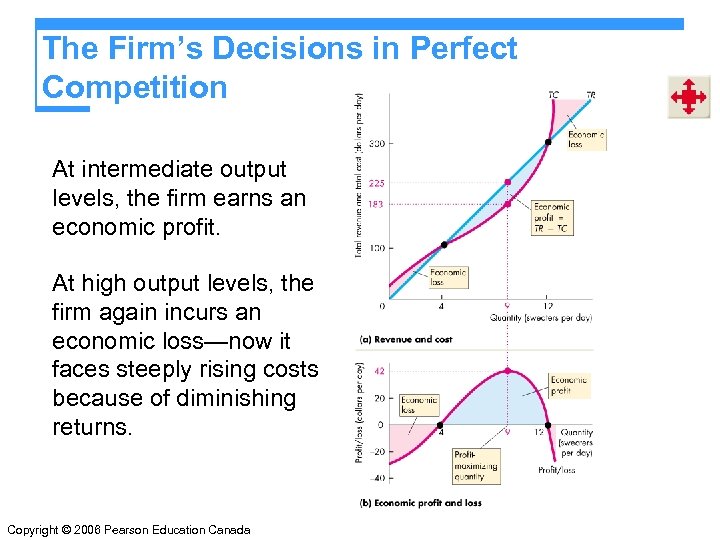The Firm’s Decisions in Perfect Competition At intermediate output levels, the firm earns an economic profit. At high output levels, the firm again incurs an economic loss—now it faces steeply rising costs because of diminishing returns. Copyright © 2006 Pearson Education Canada

The Firm’s Decisions in Perfect Competition Marginal Analysis The firm can use marginal analysis to determine the profitmaximizing output. Because marginal revenue is constant and marginal cost eventually increases as output increases, profit is maximized by producing the output at which marginal revenue, MR, equals marginal cost, MC. Figure 11. 3 on the next slide shows the marginal analysis that determines the profit-maximizing output. Copyright © 2006 Pearson Education Canada

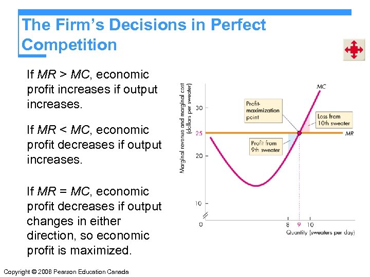The Firm’s Decisions in Perfect Competition If MR > MC, economic profit increases if output increases. If MR < MC, economic profit decreases if output increases. If MR = MC, economic profit decreases if output changes in either direction, so economic profit is maximized. Copyright © 2006 Pearson Education Canada

The Firm’s Decisions in Perfect Competition Profits and Losses in the Short Run Maximum profit is not always a positive economic profit. To determine whether a firm is earning an economic profit or incurring an economic loss, we compare the firm’s average total cost, ATC, at the profit-maximizing output with the market price. Figure 11. 4 on the next slide shows the three possible profit outcomes. Copyright © 2006 Pearson Education Canada

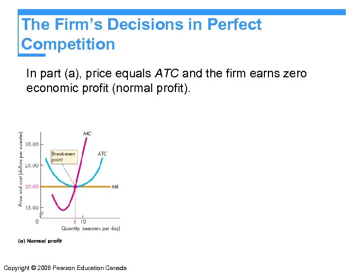The Firm’s Decisions in Perfect Competition In part (a), price equals ATC and the firm earns zero economic profit (normal profit). Copyright © 2006 Pearson Education Canada

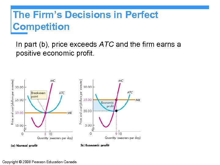The Firm’s Decisions in Perfect Competition In part (b), price exceeds ATC and the firm earns a positive economic profit. Copyright © 2006 Pearson Education Canada

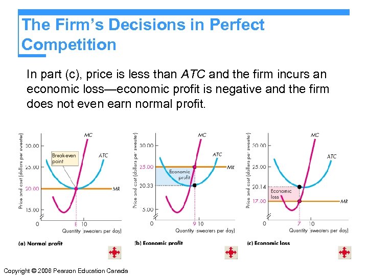The Firm’s Decisions in Perfect Competition In part (c), price is less than ATC and the firm incurs an economic loss—economic profit is negative and the firm does not even earn normal profit. Copyright © 2006 Pearson Education Canada

The Firm’s Decisions in Perfect Competition The Firm’s Short-Run Supply Curve A perfectly competitive firm’s short-run supply curve shows how the firm’s profit-maximizing output varies as the market price varies, other things remaining the same. Because the firm produces the output at which marginal cost equals marginal revenue, and because marginal revenue equals price, the firm’s supply curve is linked to its marginal cost curve. But there is a price below which the firm produces nothing and shuts down temporarily. Copyright © 2006 Pearson Education Canada

The Firm’s Decisions in Perfect Competition Temporary Plant Shutdown If price is less than the minimum average variable cost, the firm shuts down temporarily and incurs a loss equal to total fixed cost. This loss is the largest that the firm must bear. If the firm were to produce just 1 unit of output at a price below average variable cost, it would incur an additional (and avoidable) loss. Copyright © 2006 Pearson Education Canada

The Firm’s Decisions in Perfect Competition The shutdown point is the output and price at which the firm just covers its total variable cost. This point is where average variable cost is at its minimum. It is also the point at which the marginal cost curve crosses the average variable cost curve. At the shutdown point, the firm is indifferent between producing and shutting down temporarily. It incurs a loss equal to total fixed cost from either action. Copyright © 2006 Pearson Education Canada

The Firm’s Decisions in Perfect Competition If the price exceeds minimum average variable cost, the firm produces the quantity at which marginal cost equals price. Price exceeds average variable cost, and the firm covers all its variable cost and at least part of its fixed cost. Copyright © 2006 Pearson Education Canada

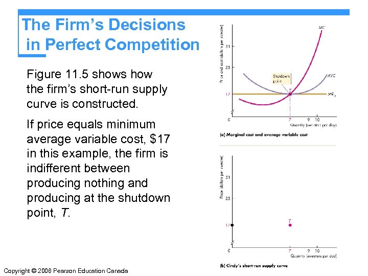The Firm’s Decisions in Perfect Competition Figure 11. 5 shows how the firm’s short-run supply curve is constructed. If price equals minimum average variable cost, $17 in this example, the firm is indifferent between producing nothing and producing at the shutdown point, T. Copyright © 2006 Pearson Education Canada

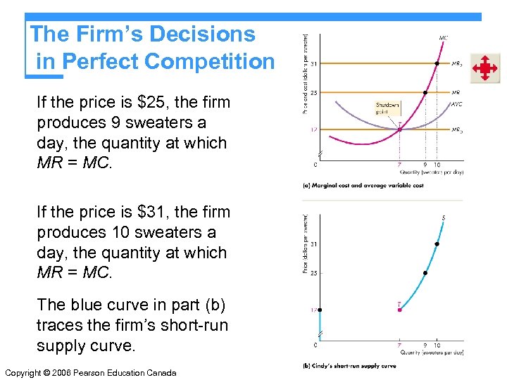The Firm’s Decisions in Perfect Competition If the price is $25, the firm produces 9 sweaters a day, the quantity at which MR = MC. If the price is $31, the firm produces 10 sweaters a day, the quantity at which MR = MC. The blue curve in part (b) traces the firm’s short-run supply curve. Copyright © 2006 Pearson Education Canada

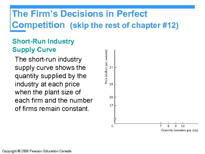The Firm’s Decisions in Perfect Competition (skip the rest of chapter #12) Short-Run Industry Supply Curve The short-run industry supply curve shows the quantity supplied by the industry at each price when the plant size of each firm and the number of firms remain constant. Copyright © 2006 Pearson Education Canada